Author's Response
The Popperian
framework, statistical significance, and Rejection of Chance
Siu L. Chow
Department of Psychology, University of
Regina, Regina, Saskatchewan, Canada S4S OA2.
siu.chow@uregina.ca uregina.ca/chowsl/
Abstract: That Haig and Sohn
find the hypotheticodeductive approach wanting in different
ways shows that multiple conditional syllogisms are being used
in different stages of' theory corroboration in the Popperian
approach. The issues raised in the two commentaries assume a different
complexion when certain distinctions are made.
Separate conditional syllogisms at different
levels of abstraction are being used to justify the rejection
of chance in significance tests and to corroborate theories. Haig's
concerns are met with a discussion of the nature of psychometric
instruments, the incommensurability problem of meta-analysis,
and the circularity of adductive conclusions. Simulation data
are used to answer Sohn's critiques by showing that (a)
the alpha level is not meant to be applied to a set of ttests,
and (b) statistical significance is dependent on neither effect
size nor sample size.
It is important to calibrate an instrument
if it is used to obtain exact measurements (e.g., a clock). Psychologists
do not use significance tests for calibration purposes because
psychometric instruments provide relative, not absolute, measurements.
For example, a WISCR score of 115 indicates, not how intelligent
an individual is, but that the individual is better than 84.13%
of the norm group. The acceptability of a psychometric instrument
depends on its validity, not the sort of precision monitored by
calibration.
The 12 studies described in Chow's (1996)
Table 5.5 belong to the same domain. To conduct a metaanalysis
on them is to obtain the average of the diverse effects of the
qualitatively different independent variables. The result is conceptually
anomalous because it is not theoretically meaningful to mix apples
and oranges. As no valid conclusion can be drawn from metaanalysis,
it cannot be used to discover new phenomena.
Haig's concerns
about theory discovery and the interrelationships among phenomenon,
theory, and evidential data have been anticipated in Sections
3.2.1 (pp. 4647) and 3.7 (pp. 6364) in Chow (1996).
Given the "phenomenon hypothesis evidential data" sequence
(Chow 1996, pp. 46 & 63), the theory is necessarily an
ad hoc postulation visàvis the
tobeexplained phenomenon. It is circular for Haig
to assert that "phenomena provide the evidence for theories."
Hence, theories obtained by adduction, like theories established
by any other means, have to be corroborated. A series of three
embedding conditional syllogisms is used when corroborating theories,
including adductively established ones (Chow 1996, Table 4.2,
p. 70).
The null hypothesis (H0) is used
in significance tests as the antecedent and the consequent of
two conditional propositions (Chow 1996, p. 32) as follows:
[Proposition 1]: If the research manipulation
is not efficacious (i.e., only chance influences are assumed),
then H0.
[Proposition 2]: If H0,
then the mean difference of the sampling distribution of
differences is zero.
This practice of emphasizing that H0
is an implication of the chance hypothesis, not the chance hypothesis
itself, will henceforth be called the formal approach. Sohn's
treatment of H0 as the chance hypothesis is acceptable
as a casual way to express the transitive relationship between
Propositions 1 and 2. Subsequently, it is called the vernacular
approach.
There are important differences between the
formal and vernacular stances. For example, Proposition 2 is true
only if Ho is the zeronull (i.e., H0:
u1 = u2). If H0
is a pointnull (e.g., u1 - u2
= 5), Proposition 2 is replaced by Proposition 3:
[Proposition 3]: If H0:
u1 - u2 = 5, then the
mean difference of the sampling distribution of differences is
5.
Not making the distinction between the formal
and vernacular approaches is responsible for some of the issues
raised by Sohn.
If H0 were the chance hypothesis,
"significant" and "rejecting the chance hypothesis"
become synonymous characterizations. The question about justification
becomes mute because two synonymous expressions do not (and cannot)
have a justificatory relationship. On the other hand, excluding
chance as an explanation by rejecting H0 in the case
of Proposition 1 is warranted by modus tollens (Chow 1996,
pp. 5052).
Sohn questions
the justificatory function of modus tollens because of
Berkson's (1942) conditional syllogism. If one were to
follow Berkson's example, A represents the chance hypothesis,
and B stands for H0, This is not possible when H0
is the chance hypothesis (viz., Sohn's contention), however, because
a concept does not imply itself. Moreover, the "sometimes"
qualifier makes ambiguous Berkson's major premise. Furthermore,
there is a confusion in Sohn's appeal to Berkson.
[Proposition 4]: Of all possible differences
between 2 sample means, 5% produce a tvalue equal
to, or smaller than, the critical t value.
[Proposition 5]: Some differences between
two sample means produce a t value equal to, or smaller
than, the critical t value.
Proposition 4 is a definite statement
about a probabilistic phenomenon that can be tested. The ambiguity
of Berkson's (1942) minor premise (like Proposition 5)
precludes it from being used as a criterion for making the statistical
decision. Subscribing to Berkson's reasoning betrays a confusion
between adopting a welldefined probabilistic statement and
using a vague proposition.
Sohn finds
the reasonableness of the formal approach wanting because one
can never be certain that H0 is false when one rejects
it. This objection would be unassailable if absolute certainty
were the prerequisite for reasonableness. Be that as it may, the
inevitable uncertainty in question does not invalidate the formal
approach.
The Type I error becomes a concern when there
are reservations about the statistical significance of the result
of a specific experiment. Such is an occasion for checking the
correctness of the experimental hypothesis, the presence of a
confounding variable, or the appropriateness of the experimental
design, task or procedure. That is, instead of disputing the validity,
usefulness or importance of significance tests, the inevitable
uncertainty serves to ensure conceptual or methodological rigor.
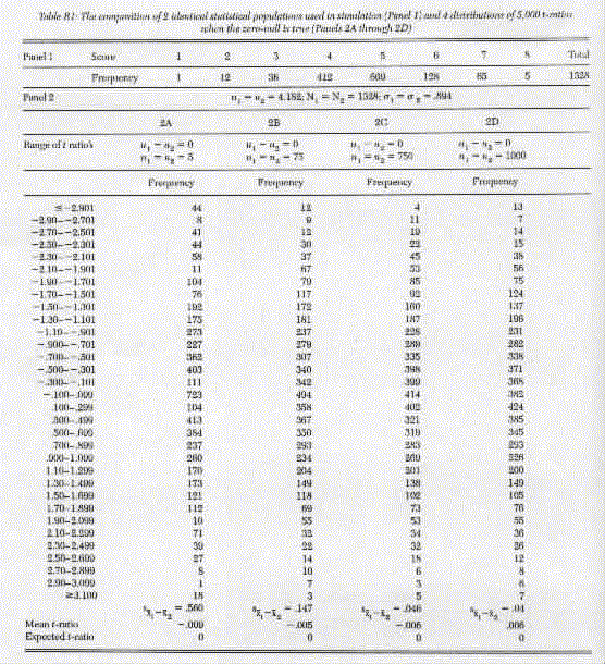
Sohn's two scenarios set in high relief a common misunderstanding about significance tests. Specifically, it is said in the first scenario (Sohn's para. 5) that, given a = .05, the results of around 50 of 1,000 separate ttests will be significant by chance when the zeronull hypothesis is true. This statement is as incorrect as saying that there will be n heads and n tails in 2n identical tosses of a fair coin. What a fair coin implies is that 50% of an infinite number of identical tosses result in heads. It does not follow that half of any exact number of identical tosses will result in heads. Consider the first scenario more closely with reference to Table R1.

Underlying the ttest are two statistical populations specified by the two levels of the independent variable (Winer 1962). Shown in Panel 1 of Table R1 is the composition of two such populations. Their means are shown in Panel 2 (viz., u1 = u2 = 4.812) and they have the same standard deviation (viz., (s1 = s2 =.894). The following steps were carried out:
(a) Selected with replacement a random sample of n units from Population 1 and another random sample of n, from Population 2, and n1 = n2.
(b) Ascertained the difference between the two sample means, as well as the standard error of the difference.
(c) Calculated the t ratio.
(d) Returned the two sets of n units to their respective populations.
(e) Repeated Steps (a) through (d) 5,000 times.
(f) Steps (a) through (e) were repeated with
u1 = u2 = 5, 75, 750, and
1,000.
Given any sample size, there are 5,000 differences
at the end of the exercise. When they are tabulated in the form
of a frequency distribution, the result is an empirical approximation
to the random sampling distribution of the differences between
two sample means. It is only an approximation because, in theory,
Step (e) should consist of an infinite number of times.
The 5,000 tvalues obtained in
Step (c) represent the result of standardizing the 5,000 differences
in terms of their respective standard errors of differences. Shown
in Column 2A of Table R1 are the numbers of empirically
determined tvalues that fall within the ranges identified
in the corresponding row. For example, 104 tvalues
fall between 1.90 and 1.701. This simulation
exercise is to make explicit four points:
(1) The probability foundation of the ttest is the sampling distribution of differences.
(2) A different sampling distribution of differences is used when the sample size changes (see Columns 2A through 2D of Table R1).
(3) The expression "a = .05" means that 5% of an infinite number of differences between 2 means give tvalues that are as extreme as, or more extreme than, 1.86 (or 1.86 as the case may be) for the 1tailed test with (df = 8.
(4) It does not follow from (3) that
5% of any 1,000 differences would be as extreme as, or
more extreme than, the critical t value.
To recapitulate (1), every application of
the ttest evokes the appropriate sampling distribution of
differences. Hence, the same sampling distribution is evoked 1,000
times in Sohn's first scenario if the 2 statistical
populations (as well as n1 and n2)
remain the same throughout. The 50-950 split of the 1,000 experiments
envisioned by Solin has nothing to do with the alpha level for
the reasons stated in (3) and (4).
Given that testing a pointnull hypothesis
is no different from testing a zeronull hypothesis (Kirk,
1984), the outcomes of significance tests should be independent
of the expected effect size (Chow, 1996, pp. 132-34; 1998a, pp.
18485). This contradicts the second scenario described in
Sohn's paragraph six, which is an echo of the poweranalytic
"significanceeffect size dependence" assertion
that the outcomes of significance tests depend on effect size
(Cohen, 1987). This point is amplified below.
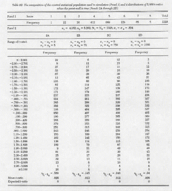
The entries in Table R2 were also obtained with Steps (a) through (f), except that mean of the second statistical population is larger than that of the first one by 0.5 of the standard deviation of the first statistical population (viz., u1 = 4.812; u2 = 5.262; Panel 2). If the "significanceeffect size dependence" thesis were correct, the mean tratio should differ from zero. There is no support for the "significanceeffect size dependence" thesis because none of the four mean tratios differs from 0 (viz., .028, .013, .012, and .008).

Sohn's second scenario also echoes another poweranalytic assertion, namely, that larger sample sizes increase statistical power, thereby making it easier to obtain statistical significance. This "significancesample size dependence" thesis is questioned by the four c2 tests reported in the two panels of Table R3, as may be seen from the italicized and boldface entries in the two panels.

Use Panel B of Table R3 as an illustration.
Each of the 5,000 tvalues in Column 2A of Table R2
was classified as "Significant" or "Not significant."
For example, there are 456 and 4544 tvalues
in the "Significant" and "Not significant"
categories, respectively, when n1 = n2
= 5. The same process was repeated with the entries from each
of the other columns of Table R2 (i.e., for sample sizes
of 75, 750, and 1,000). The result is the eight boldface
entries in Panel B of Table R3. They make up the twoway
c2
test for the independence of statistical significance (columns)
and sample size (rows). As the c2
= 2.64 (df = 3) is not significant, there is no
reason to reject the independence in question. That is, there
is no support for the view that statistical significance is a
function of sample size in the case of the point-null.
The procedure just described was also curried
out with the entries of Table R1. The result is the eight italicized
entries in Panel A of Table R3. The c2
of 2.93 (df = 3) is also not significant. Hence, there
is also no support for the "significancesample size
dependence" thesis in the case of the zeronull.
To conclude, it is necessary to distinguish
between (a) phenomenon and evidential data, and (b) the chance
hypothesis and H0. The inevitable possibility of committing
the Type I error does not invalidate the formal approach to significance
tests. The exclusion of the chance explanation by rejecting H0
is warranted by modus tollens. Although the critical tvalue
defined by the alpha level serves as the decision criterion in
every ttest, it has nothing to do with a collection
of separate ttests as a set.
References
Letters "u" and "r"
appearing before authors' initials refer to target article and
response respectively
Baird, D. (1992) Inductive logic: Probability and statistics. Prentice Mill. [BDH]
Berkson, J. (1942) Tests of significance considered as evidence. Journal of the American Statistical Association 37:32535. [DS]
Chow, S. L. (1996) Statistical significance: Rationale, validity, and utility. Sage, [rSLC, BDH, DS] BDH, DS]
(1998a) Précis of Statistical significance Rationale, validity. and utility. Behavioral and Brain Sciences 21:169239. [rSLC, DS]
(1998b) The nullhypothesis significancetest procedure is still warranted. Behavioral and Brain Sciences 21:22838. [BDH]
Cohen, J. (1987) Statistical power analysis for the behavioral sciences (revised edition). Academic Press. [rSLC]
Erwin, E. (1998) The logic of null hypothesis testing. Behavioral and Brain Sciences 21:19798. [BDH]
Franklin, A. (1997) Calibration. Perspectives on Science 5:3180. [BDH]
Hunter, J. E. (1998) Testing significance testing: A flawed defense. Behavioral and Brain Sciences 21:204. [BDH]
Josephson, J. R. & Josephson, S. G., eds. (1994) Abductive inference. Cambridge University Press. [BDH]
Kirk, R. E. (1984) Basic statistics, 2nd edition. Brooks/Cole. [rSLC]
Nickles, T (1987) Methodology, heuristics and rationality In: Rational changes in science, ed. J. C. Pitt & M. Pera. Reidel. [BDH]
Schmidt, F L. (1992) What do data really mean? Research findings, meteanalysis, and cumulative knowledge in Psychology. American Psychologist 47:117381. [BDH]
Sohn, D. (1993) Psychology of the scientist: LXVI. The idiot savants have taken over the Psychology labs! Or why in science the rejection of the null hypothesis as the basis for affirming the research hypothesis is unwarranted. Psychological Reports 73:116775. [DS]
Thagard, P. (1992) Conceptual revolutions, Princeton University Press. [BDH]
Winer, B. J. (1962) Statistical principles in experimental design, McGrawHill. [rSLC]
Woodward, J. (1989) Data and phenomena. Synthese
79:393472.[BDH]