
|
University of Southampton Institute of Transducer Technology |
Using Artificial Neural Networks to Determine the Impulse Response of Sensors |
Dynamic measurement is an important requirement in many situations. The application of the measurand to the raw sensor results in a transient output waveform that can sometimes take a considerable time to settle sufficiently before a stable measurement is achievable. Dynamic measurement requires the system to determine the final value of the measurand before the transient effects have decayed. Classical signal processing techniques such as adaptive filter can be used to reduce dramatically the effect of oscillation in the sensor signal. New approaches however, are required when the transducer senses the measurand for only very short period. Usually the sensor signal has a few key features that are unique for any input and they can be extracted from a small portion of the signal. For example the period and the amplitude of first peak and trough. Therefore, the sensor can be envisaged as a function that maps the physical input to the output key features. Having the inverse function and extracting the key features make it possible to determine the input shortly after stimulating the sensor. Neural networks are a good candidate for implementing the inverse function of the sensor because some types have the capability of approximating any continuous function with an arbitrary accuracy subject to have sufficient neurones. In addition they can learn the behaviour of the sensor from some experimental data, so there is no need for modelling the sensor characteristics. They also have the property of generalisation, which means they are able to correctly map inputs that they have not been exposed to during the training phase.
To establish theoretical and experimental basis for the proposed method, system simulation was carried out on a tri-beam load cell, a highly resonant mechanical force sensor. Figure 1 shows the diagram of this device. It is based on thick-film technology, therefore offering advantages of cheapness and robustness. The structure is planar and produced by an inexpensive process of stamping out a steel shape and then printing it with strain gauges and conductors. The cell consists of three beams joined and supported at the centre with three pins near their extremities supporting the weigh pan. Thick-film strain gauges are screen printed onto the structure on both sides of beams. The twelve piezoresistors are connected in bridge arrangement and the interconnection is achieved through thick film conductor. A connection is made from one side of the beam to other by a wire link.
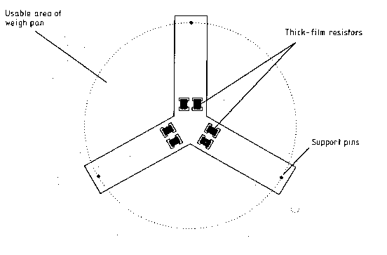
Figure 1 - Diagram of the tri-beam load cell. The planar cell is supported at the centre and pins on the arms support the weigh pan
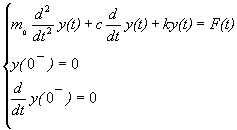
The tri-beam load cell is a highly resonant structure. The general equation for the dynamic response of this sensor is given by the following equation:
Where m0 is the effective mass of the sensor, c is the damping factor, k is the spring constant, F(t) is the force function and y(0-) and dy(0-)/dt show the initial position and the initial velocity of the platform, respectively. From the experimental data, the constants in equation set (1) were found to be c=3.5 and k=27000.
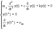
If a mass drops onto the load cell from a fixed height, h, and bounces clear, so it is in contact with the load for a very shot period, then the input function can be written as F(t)=Md(t), where M is a constant that depends on m and d(t) is the unit impulse function. Equation (1) can be written as follows for t>0 because the impulse function is zero for t>0 and its effect only changes the initial conditions.
where v2a is a constant. To calculate this constant suppose v1 shows the speed of load just before collision, v1a shows the speed of load just after collision, v2 shows the speed of the sensor plate just before collision and v2a shows the speed of the sensor plate just after collision.
If the load falls from the height of h with zero initial velocity then v1=(2gh)1/2 where g is the gravitational constant. The sensor plate is at rest initially hence v2=0. Newton's Second law implies mv1+m0v2=mv1a+m0v'2a where m shows the mass of the load. By definition the restitution coefficient, e, is given by (3):
|
|
(3) |
e=1 refers to an elastic impact ( impact with no energy loss ) and e=0 indicates inelastic or plastic impact. Using this information v2a can be calculated as (4):
|
|
(4) |
Knowing v2a, the solution for equation (2) can be written as (5)
|
|
(5) |
Where a=c/m0, wn2=k/m0, wd=(wn2-a2)1/2 and a, wd and wn are the damping ratio, the damped frequency and the natural frequency respectively.
Equation (5) shows that the amplitudes of peaks and troughs only depend on the magnitude of m. if the loads fall from a fixed height. This equation is used for simulation of the sensor signal. In reality the signal is always contaminated by noise, therefore a normal random sequence with zero mean and variance equate to 2 percent of the mass was added to the signal. The first peak and trough of the signal were extracted as two key features and a Radial Basis Function (RBF) neural network was used to perform the inverse function approximation. To train the neural network 10 patterns are used. These patterns were generated by choosing masses that were uniformly distributed over the range of 1 to 12 g. For testing purposes patterns were generated by choosing masses that were different from those used for training. The result of the test is shown in Figure 2. It shows that the maximum error is less than 0.35%.
From the results it can be concluded that the Neural networks can be used successfully for determining the impulse response of sensors with a highly resonant structre. There is no need for system identification and sensor modeling. The neural networks learn the behavior of the sensor from the set of training patterns. Using a pre-processing block before neural network dramatically reduces the number of neurones. This, in turn reduces the complexity of computation and offers the possibility of a very fast measurement.
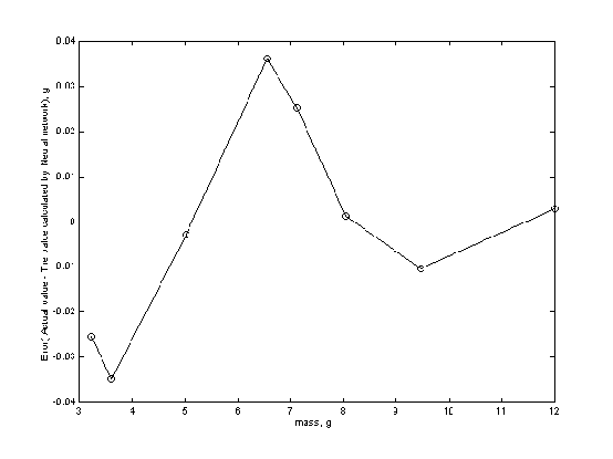
Figure 2 . The output of neural network and the corresponding error
|
![[Uni. Home]](images/unilogo.gif)