optimisationTilePlot

Tile plot of four dimensions of a problem

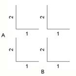
This plots the behaviour of the objective function over four dimensions of a problem. The first two of the design variables (A and B) are plotted across rows and columns of tiles. The third and fourth design variables (1 and 2) will be plotted across the x and y axes of each tile.

Each design variable will be sampled at the specified number of points between the limits defined within the fields LVARS and UVARS of STRUCTIN. For example a problem in which the variables A and B are each sampled at two points the resulting tile plot will have four tiles.

The value of the objective function is plotted as a surface within each 2D tile. The surface colormap is consistent between the tiles. The tile plot is interactive, and by clicking on a tile it is visible as a 3D plot in a separate figure window.

Syntax

optimisationTilePlot(STRUCTOUT,STRUCTIN,DESIGNVARS, NUMPOINTS,TILETYPE)

optimisationTilePlot(...,PLOTPOINTS)

optimisationTilePlot(...,FIG)

FIG = optimisationTilePlot(...)

[FIG,TILESOUT,TILESIN] = optimisationTilePlot(...)

optimisationTilePlot(TILESOUT,TILESIN)

Description

optimisationTilePlot(STRUCTOUT,STRUCTIN,DESIGNVARS, NUMPOINTS,TILETYPE) where STRUCTOUT is the results structure returned by OptionsMatlab and STRUCTIN is the corresponding OptionsMatlab input structure. If the TILETYPE is direct search STRUCTOUT can be empty [].

DESIGNVARS must be a four element vector that defines the design variables to be plotted [A,B,1,2] based upon their index in STRUCTIN.VARS. NUMPOINTS must also be a four element vector that defines the number of points to be evaluated for each of the DESIGNVARS.

TILETYPE is an integer that defines how the tile is to be evaluated. The valid values of TILETYPE are:

1 = Evaluation of the RSM defined by the fields OBJMOD and CONMOD of STRUCTIN

2 = Direct search of the objective function

optimisationTilePlot(...,PLOTPOINTS) as above when PLOTPOINTS is a flag that indicates whether to plot the data points. For a RSM if

PLOTPOINTS = 1 the original data points contained in STRUCTOUT will be plotted in each tile, otherwise for a direct search the evaluated points will be plotted. If

PLOTPOINTS = 0 the points will not be plotted. Default value PLOTPOINTS = 0.

optimisationTilePlot(...,FIG) as above where FIG is the figure in which to plot the tile plot. If FIG is not provide a new figure will be generated. FIG can also be empty [].

FIG = optimisationTilePlot(...) as above where FIG is a the number of figure in which the tiles were plotted.

[FIG,TILESOUT,TILESIN] = optimisationTilePlot(...) as above where TILESOUT and TILESIN are cell arrays containing the OptionsMatlab output and input structures that were used to generate the surfaces for each of the tiles.

optimisationTilePlot(TILESOUT,TILESIN) replots the tile plot with data returned in the cell arrays TILESOUT and TILEIN. All other input arguments are optional. The PLOTPOINTS argument can be supplied to indicate that the data points should be plotted.

Examples

The following example demonstrates a tile plot of the peaks4d problem using direct search:

>> structin = createpeaks4dstruct(2.8);

>> optimisationTilePlot([],structin,[3,4,1,2],[2,3,15,15],2)

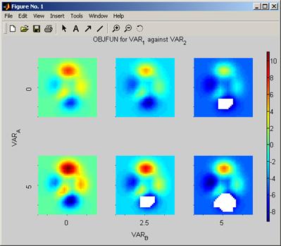
Figure 16 Tile plot of the peaks4d problem produced by direct search

By clicking on the tiles of the tile plot with the mouse that tile will be displayed in 3D. For example by clicking on the tile in the top left of the figure the following plot will be displayed:

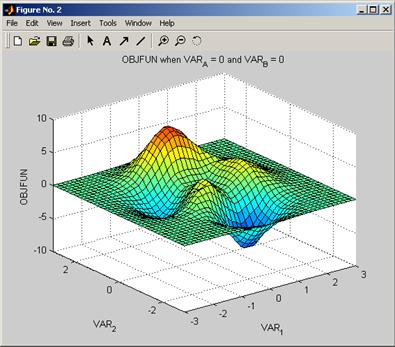
Figure 17 Tiles may be viewed in 3D by clicking on the tile plot

The second example demonstrates a tile plot of the peaks4d problem produced using a Shepard RSM. Using the PLOTPOINTS argument the points of the original data set are also plotted:

>> structin = createpeaks4dstruct(2.8);

>> structin.NITERS = 25;

>> structout = OptionsMatlab(structin);

>> structin.OBJMOD = 1; %Shepard RSM

>> structin.CONMOD = 1;

>> optimisationTilePlot(structout,structin,[3,4,1,2], [2,3,15,15],1,1)

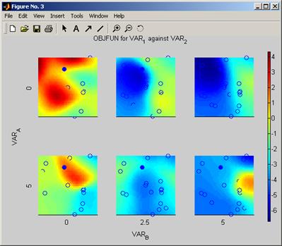
Figure 18 Tile plot of the peaks4d problem produced with a Shepard RSM and the original data set