Builds and samples a Response Surface Model.

 

This function will generate an array of candidate points and then invokes OptionsMatlab to build a Response Surface Model (RSM) and samples the candidate points. The structure returned by optimisationSampleRSM can then be plotted.

 

Syntax

STRUCTOUT = optimisationSampleRSM(STRUCTIN,RESULTS, NUMPOINTS)

STRUCTOUT = optimisationSampleRSM(...,LVARS,UVARS)

[STRUCTOUT, VECTORS] = optimisationSampleRSM(...)

 

Description

STRUCTOUT = optimisationSampleRSM(STRUCTIN,RESULTS, NUMPOINTS) where STRUCTIN is an OptionsMatlab input structure which specifies the RSM, and RESULTS is an output structure containing the results over which the RSM is built. If NUMPOINTS is a scalar value, this will specify the total number of sample points which will be distributed evenly across NVRS dimensions.  Otherwise NUMPOINTS must be a vector of length NVRS which specifies the number of sample points in each dimension (the total number of sample points will equal PROD(NUMPOINTS) ). The return argument STRUCTOUT will contain the output structure returned by OptionsMatlab.

 

To hold a design variable constant set the corresponding element of NUMPOINTS equal to zero. All design variables for which NUMPOINTS is zero will be sampled at the value specified by STRUCTIN.VARS.

 

STRUCTOUT = optimisationSampleRSM(...,LVARS,UVARS) as above where LVARS and UVARS are vectors that specify the upper and lower limits between which the design variables are sampled. If these vectors are not specified the values of LVARS and UVARS defined in STRUCTIN are used.

 

[STRUCTOUT, VECTORS] = optimisationSampleRSM(...) as above where VECTORS is a cell array containing NVRS vectors of the points at which the each of the design variables were sampled. 

 

Examples

The first example will sample response surface models built over the beam problem.

 

%Run a DOE in OptionsMatlab

input1 = createBeamStruct;

input1.NITERS = 50;

output1 = OptionsMatlab(input1);

 

%Create an input structure to search a RSM

input2 = createBeamStruct;

input2.OBJMOD = 3.3;     

input2.CONMOD = 3.3;       

 

%Sample 100 evenly spaced points

output2 = optimisationSampleRSM(input2, output1, 100)

 

 

%Plot an interpolated surface over the sampled points

fig = optimisationTerrain(output2, input2);

%Plot the original points

optimisationTrace(output1, input1, 1, fig);

 

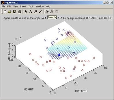
Figure 8 First plot of the output of optimisationSampleRSM

 

%Sample 5 points in the first dimension and 20 points in the

%second dimension

output3 = optimisationSampleRSM(input2, output1, [5, 20])

optimisationTerrain(output3, input2);

 

 

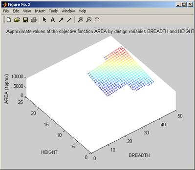
Figure 9 Second plot of the output of optimisationSampleRSM

 

The second example samples the bump problem over two dimensions of a five dimensional problem. The values of the design variables which are held constant are specified by input5.VARS.

 

%Run a DOE over the bump function in 5 dimensions

input4 = createbumpstruct(2.8, 5);

input4.NITERS = 50;

output4 = OptionsMatlab(input4);

 

%Build a RSM over the DOE and sample in the second and third

%dimensions

input5 = createbumpstruct(2.8, 5);

input5.OBJMOD = 3.3;

input5.CONMOD = 3.3;

output5 = optimisationSampleRSM(input5,output4,[0,20,20,0,0]);

 

%Plot the sampled points in the second and third dimensions

optimisationTerrain(output5, input5, 1, [], [-37.5,30], [2,3]);

 

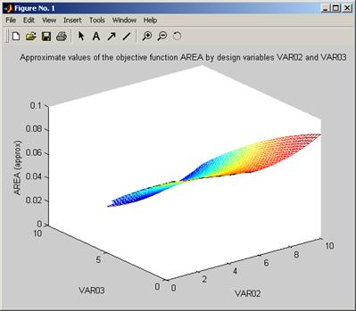
Figure 10 Third plot of the output of optimisationSampleRSM

 

See also

optimisationTerrain, OptionsMatlab

 

Copyright © 2007, The Geodise Project, University of Southampton