5 Frequently Asked Questions
5.1 Why does Matlab crash when I call OptionsMatlab?
When OptionsMatlab is invoked with an invalid Gendat license file the error message below will be printed:
>> input = createBeamStruct;
>> output = OptionsMatlab(input);
??? Optimization failed. OPTIONS Error code: -2147483648
Gendat license files may be invalid if they have expired, or if they contain incorrect machine details.
Write statements by some of the third party algorithms available within the Options have also caused OptionsMatlab to crash. These can be diagnosed by examining the temporary files generated by OptionsMatlab; .OPTIONS*.opt and .OPTSDTO*.opt. In some cases this behaviour can be ameliorated by reducing the output level of OptionsMatlab, OLEVEL = 0.
When creating a new problem definition conflicts between user-specified design variable, parameter or constraint names can cause OptionsMatlab to crash. Conflicts occur when there is an ambiguity between a variable name and the name of an existing Options variable. For example the variable name FACT would be ambiguous if the parameter FACTOR had previously been defined. If a variable name conflict has caused Matlab to crash this may be diagnosed by examining the temporary file .OPTIONS*.opt.
Please report any reoccurring problems to me by email. Bugs are documented in the buglists included in the OptionsMatlab distribution.
5.2 How do I specify the search method?
The search method is specified by the field OMETHD of the Options input structure. The scalar values correspond to the search methods listed below. For more details of each of the search methods please see the Options manual [1].
0.0 to just evaluate the user’s problem code at the point specified
1.1 for OPTIVAR routine ADRANS
1.2 for OPTIVAR routine DAVID
1.3 for OPTIVAR routine FLETCH
1.4 for OPTIVAR routine JO
1.5 for OPTIVAR routine PDS
1.6 for OPTIVAR routine SEEK
1.7 for OPTIVAR routine SIMPLX
1.8 for OPTIVAR routine APPROX
1.9 for OPTIVAR routine RANDOM
2.1 for user specified routine OPTUM1
2.2 for user specified routine OPTUM2
2.3 for NAG routine E04UCF
2.4 for bit climbing
2.5 for dynamic hill climbing
2.6 for population based incremental learning
2.7 for numerical recipes routines
2.8 for design of experiment based routines
3.11 for Schwefel library Fibonacci search
3.12 for Schwefel library Golden section search
3.13 for Schwefel library Lagrange interval search
3.2 for Schwefel library Hooke and Jeeves search
3.3 for Schwefel library Rosenbrock search
3.41 for Schwefel library DSCG search
3.42 for Schwefel library DSCP search
3.5 for Schwefel library Powell search
3.6 for Schwefel library DFPS search
3.7 for Schwefel library Simplexsearch
3.8 for Schwefel library Complexsearch
3.91 for Schwefel library twomembered evolution strategy
3.92 for Schwefel library multimembered evolution strategy
4 for genetic algorithm search
5 for simulated annealing
6 for evolutionary programming
7 for evolution strategy
5.3 How do I run a Design of Experiments?
A Design of Experiments search can be used to efficiently sample points across the multi-dimensional parameter space represented by large numbers of design variables. A Design of Experiments search can be invoked by setting OMETHD = 2.8. The number of points to be evaluated can be configured by altering the input structure field NITERS.
A number of different Design of Experiments search methods are available within the Options package. These can be configured using the optional input field MC_TYPE, where;
1 Random (default)
2 LPt
3 Central composite and LPt
4 Full factorial and LPt
5 Latin hypercubes
6 Cell-based latin hypercubes
7 User supplied candidate points
For more details about these Design of Experiments search methods please consult the Options manual [1].
User supplied candidate points to be evaluated during a Design of Experiments can be supplied with the optional input field DOE_TRACE when the control parameter MC_TYPE = 7. DOE_TRACE requires two mandatory fields:
DOE_TRACE.NCALLS containing the number of user-supplied DOE points
DOE_TRACE.VARS the design points to be evaluated during the DOE (size NVARS by DOE_TRACE.NCALLS)
When using user supplied candidate points NITERS must equal DOE_TRACE.NCALLS plus one as the Design of Experiments will first evaluate the design point specified by VARS.
5.4 How do I build a Response Surface Model?
A Response Surface Model is used to approximate the value of objective or constraint functions based upon the results of direct evaluation of the user’s model. Response Surface Models can be built independently over the objective and constraints, and are configured using the optional input fields OBJMOD and CONMOD respectively. If these fields are not set OptionsMatlab will directly evaluate the user supplied objective and constraint functions.
A number of Response Surface Model methods are available to be used to approximate the values of the objective function and constraints. The possible settings for the optional input fields OBJMOD and CONMOD are:
1.0 for a Shepard response surface model
2.1 for linear Radial Basis Function
2.2 for thin plate Radial Basis Function
2.3 for cubic splines Radial Basis Function
2.4 for cubic splines Radial Basis Function with regression via reduced bases
3.1 for mean polynomial regression model
3.2 for first order polynomial regression model
3.3 for first order polynomial regression model plus squares
3.4 for first order polynomial regression model plus products (crossterms)
3.5 for second order polynomial regression model
3.6 for second order polynomial regression model plus cubes
4.1 for a Stochastic Process Model
4.2 for the root mean square error of the Stochastic Process Model
4.3 for the expected improvement of the Stochastic Process Model
4.31 for the expected improvement of the constrained Stochastic Process Model [requires CONMOD=4.1]
4.32 for the feasibility of improvement of the constrained Stochastic Process Model [requires CONMOD=4.1]
4.33 for the probability of improvement of the Stochastic Process Model
0.0 if the underlying user supplied function is to be called.
5.5 How do I plot my Response Surface Model?
Following OptionsMatlab version 0.9.0+ search histories are available for optimisations which are run over a Response Surface Model in the output structure field RSMTRC. Previously OptionsMatlab would only return a search history when candidate points were provided.
To evaluate a factorial search of the RSM that is suitable for plotting it may be appropriate to evaluate a list of candidate points. The candidate points must be provided in a field DOE_TRACE of the input structure (see section 5.3). In versions of OptionsMatlab 0.9.0+ it is necessary to specify that the optimisation is a candidate points Design of Experiments (OMETHD=2.8, MC_TYPE=7).
>> %Create the initial dataset
>> DOEinput = createBeamStruct;
>> DOEoutput = OptionsMatlab(DOEinput);
>> %Define a RSM input structure
>> RSMinput = createBeamStruct;
>> RSMinput.OBJMOD = 3.3;
>> RSMinput.CONMOD = 3.3;
>> %Create a list of candidate points to be evaluated
>> ii = linspace(DOEinput.LVARS(1),DOEinput.UVARS(1),10);
>> jj = linspace(DOEinput.LVARS(2),DOEinput.UVARS(2),10);
>> [x,y] = meshgrid(ii,jj);
>> RSMinput.DOE_TRACE.VARS(1,:)= reshape(x,1,prod(size(x)));
>> RSMinput.DOE_TRACE.VARS(2,:)= reshape(y,1,prod(size(y)));
>> RSMinput.DOE_TRACE.NCALLS = prod(size(x));
>> %Define the search a candidate points DoE
>> RSMinput.OMETHD = 2.8;
>> RSMinput.MC_TYPE = 7;
>> RSMoutput = OptionsMatlab(RSMinput, DOEoutput);
>> disp(RSMoutput.RSMTRC)
OBJFUN: [1x100 double]
VARS: [2x100 double]
NCALLS: 100
CONS: [5x100 double]
LCONS: [5x100 double]
UCONS: [5x100 double]
The contents of RSMTRC can then be plotted to show the surface of the Response Surface Model.
>> optimisationTerrain(RSMoutput, RSMinput);
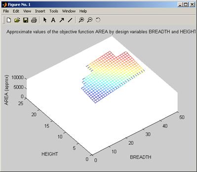
Figure 22 Plotting approximate values of the Beam objective function generated by a RSM
The utility function optimisationSampleRSM automates the process of sampling a RSM built over the user's problem.
5.6 How do I generate Design of Experiment update points?
It is possible to improve the quality of a Response Surface Model by improving to original dataset by selectively adding new points. The Genetic Algorithm (OMETHD = 4) and Dynamic Hill Climbing (OMETHD = 2.5) optimisation algorithms, when run over a Response Surface Model, are capable of returning a list of points that would improve the dataset.
Update points will be returned if the OptionsMatlab input structure contains the optional field NUMUPDATE. The value of NUMUPDATE is a scalar which determines the number of update points to be returned when a search routine is run over a RSM. The update points will be returned in the field DOE_TRACE of the output structure.
In the following example a Genetic Algorithm is run over a RSM generated from the search history contained in the structure DOEoutput. NUMUPDATE is set to equal 10, meaning that the Genetic Algorithm will suggest ten update points at which the original data set can be improved.
Note that the optimisation algorithm may return less than NUMUPDATE update points, in this case the remaining elements of DOE_TRACE.VARS will contain zeros.
>> %Create the initial dataset
>> DOEinput = createBeamStruct;
>> DOEoutput = OptionsMatlab(DOEinput);
>> %Define a RSM input structure
>> RSMinput = createBeamStruct;
>> RSMinput.OMETHD = 4;
>> RSMinput.OBJMOD = 3.3;
>> RSMinput.CONMOD = 3.3;
>> RSMinput.NUMUPDATE = 10;
>> RSMoutput = OptionsMatlab(RSMinput, DOEoutput);
>> disp(RSMoutput.DOE_TRACE)
NCALLS: 10
VARS: [2x10 double]
The update points contained in the field DOE_TRACE of the structure RSMoutput can now be used as candidate points for a second Design of Experiments study.
>> DOEinput2 = createBeamStruct;
>> DOEinput2.OMETHD = 2.8;
>> DOEinput2.MC_TYPE = 7;
>> DOEinput2.DOE_TRACE = RSMoutput.DOE_TRACE;
>> DOEinput2.NITERS = RSMoutput.DOE_TRACE.NCALLS+1;
>> DOEoutput2 = OptionsMatlab(DOEinput2);
Note that DOEinput2.NITERS must equal DOEinput2.DOE_TRACE.NCALLS plus one as the Design of Experiments will first evaluate the design point specified by DOEinput2.VARS.
5.7 How do I define an unconstrained optimisation?
From version 0.5 of OptionsMatlab onwards users do not have to define a null constraint function for unconstrained optimisation problems. To indicate that an optimisation problem is unconstrained the field NCONS should be set to 0. In this case the fields CNAM, LCONS, UCONS, CONS and OPTCON are not mandatory and will be ignored.
5.8 How do I write my own objective and constraint functions?
The default implementation of OPTJOB (optjob.m) requires user-defined objective and constraint functions to conform to well-defined interfaces. These interfaces are design to be compatible with objective and constraint functions used with the Matlab Optimization Toolbox [4].
The full function signature for the user-defined objective function is:
[eval,gd,H,PARAMS,CONS,U_CONS,L_CONS]=objfun(VARS,PARAMS, U_CONS,L_CONS,DATA)
Where eval is the value of the objective function at the design variables VARS. The objective function corresponding to this header can return the constraint values for the design point, CONS, and also alter the values of the parameters, PARAMS, and constraint limits U_CONS and L_CONS. The argument DATA contains the Matlab variable contained in the optional USERDATA field of the input structure. The parameters gd and H are relevant to the Matlab Optimization Toolbox [4] and are not used by OptionsMatlab.
NOTE: The full function signature for user-defined objective function has changed in OptionsMatlab version 0.7. In earlier versions the third optional input argument was CONS, the value of the constraints at VARS. However this feature was unreliable and has been removed. Please update objective functions that use the earlier form of the function signature.
The minimum function signature required by optjob.m is:
eval = objfun(VARS)
The full function signature for the user-defined constraint function is:
[CONS,ceq,GC,Gceq,PARAMS,U_CONS,L_CONS]=objcon(VARS,PARAMS,U_CONS,L_CONS,DATA)
Where CONS are the constraint values at the design variables VARS. The parameters ceq, GC and Gceq are relevant to the Matlab Optimization Toolbox [4] and are not used by OptionsMatlab.
Again the minimum function signature required by optjob.m is a lot smaller:
CONS = objcon(VARS)
Alternative implementations of OPTJOB may require different function signatures from user-defined objective and constraint functions. Please consult the documentation of alternative implementations of OPTJOB to confirm that your objective and constraint functions conform to the requirements.
Note that the OptionsMatlab may ignore altered values of the parameters, PARAMS, and constraint limits U_CONS and L_CONS if it is not appropriate to change them, for example during a Design of Experiments.
5.9 How do I evaluate a combined objective and constraint function?
The default implementation of OPTJOB (optjob.m) supports combined objective and constraint functions. The combined function must conform to following objective function signature;
[eval,gd,H,PARAMS,CONS,...] = objfun(VARS,...)
optjob.m will evaluate this function once when evaluating objective and constraint functions if the input fields OPTFUN and OPTCON specify the same function.
NOTE: The full function signature for user-defined objective function has changed in OptionsMatlab version 0.7. In earlier versions the third optional input argument was CONS, the value of the constraints at VARS. However this feature was unreliable and has been removed. Please update objective functions that use the earlier form of the function signature.
5.10 Can OptionsMatlab calculate function evaluations in parallel?
The standard OptionsMatlab job manager, optjob.m, will evaluate the objective and constraint functions sequentially. However a parallel job manager, optjobparallel2, is included in the OptionsMatlab distribution (this supersedes the parallel job manager optjobparallel). When your objective or constraint function is expensive and you wish to use a search method with inherent parallelism it may be more considerably efficient to use the parallel job manager.
To run the demo of parallel objective function evaluations enter the following commands:
>> input = createBeamStructParallel2
>> output = OptionsMatlab(input)
To make your objective and constraint functions available to optjobparallel2 different function signatures are required to those described in section 5.8. To evaluate the objective function the user must define two functions, the first which initiates the calculation of the objective function, and a second which determines whether the calculation has completed, and if so returns the value of the objective function.
In practice the first function could perform a Globus GRAM job submission [5] returning a handle which can be used to query the status of the job, and an application specific job ID. The second function will typically use the application specific job ID to retrieve the output of the GRAM job and parse the objective function (and optionally the values of the constraints also). The interaction between these functions is shown by Figure 23.
Figure 23 Parallel objective function evaluation in OptionsMatlab. Objfun.m is called ten times to begin the objective function evaluation at ten points. When these jobs are complete objfun_parse2.m is called ten times to retrieve and parse the results
The user-defined objective function called by optjobparallel2 to perform the job submission should conform to the following function prototype:
[RETRIEVALID] = objfun(VARS,...)
where RETRIEVALID is an identifier used to determine the status of the job, and to retrieve the results. The only mandatory input argument is VARS, the other input arguments PARAMS, U_CONS and L_CONS are all optional. This function must be specified in the OPTFUN field of the OptionsMatlab input structure.
A second retrieval function is be defined to return the value of the objective function. This function must have the same name as the job submission function appended with '_parse2'. For example when the objective function submission function is saved in the file 'objfun.m' the retrieval function must be saved in the file 'objfun_parse2.m'.
The retrieval function should conform to the following function prototype:
[EVAL,PARAMS,CONS,U_CONS,L_CONS]=objfun_parse2(RETRIEVALID)
where RETRIEVALID is the identifier returned by the job submission function. EVAL is the value of the objective function (or empty if the job has not completed). The other output arguments PARAMS, CONS, U_CONS and L_CONS are all optional. CONS is the value of the constraints.
If the value of the constraints and the objective function are returned by the same function the field OPTCON should be set to equal OPTFUN. Alternatively if the constraints are evaluated independently of the objective function the user may also define two separate functions to perform the job submission and to parse the constraints. In this case the functions indicated by the field OPTCON should conform to the following function prototypes:
[JOBHANDLE] = objcon(VARS,PARAMS,U_CONS,L_CONS)
[CONS,PARAMS,U_CONS,L_CONS] = objcon_parse2(RETRIEVALID)
5.11 How do I tune the hyper-parameters for a stochastic process model RSM?
Instead of searching the user’s problem OptionsMatlab can be used to tune the hyper-parameters for a stochastic process model RSM. This can be done by setting up the OptionsMatlab input structure as though you are going to build a RSM (see section 5.4) over an existing search history. Hyper-parameter tuning is specified by setting the input structure field TUNEHYPER equal to 1.
When TUNEHYPER is set the hyper-parameters are tuned using the search method specified by the input structure. The output structure will return the structures OBJHYPER (and/or CONHYPER where appropriate) in addition to the final value of the concentrated likelihood function which is used as the objective function OBJ_CLF (or CST_CLF). Note that the user’s problem is not searched, and no optimum for the user’s problem is returned.
To use the tuned hyper-parameters to build and search a RSM, or to further tune the hyper-parameters, the structures OBJHYPER and CONHYPER can be passed as fields in the OptionsMatlab input structure. These structures contain the hyper-parameter values, and upper and lower limits to these values.
The example below demonstrates hyper-parameter tuning by performing the following steps:
- training hyper-parameters over a data set
- refining hyper-parameters with further training
- searching a RSM with user supplied hyper-parameters
- searching a RSM with starting at the previous 'best-point'
This example uses the Beam problem.
% Build initial dataset
input1 = createBeamStruct;
input1.OMETHD = 2.8; %Design of Experiments
input1.NITERS = 50; %Number of iterations
input1.OLEVEL = 2;
input1.MC_TYPE = 4; %Full factorial DoE
output1 = OptionsMatlab(input1)
output1 =
VARS: [2x1 double]
OBJFUN: 3.6877e+003
CONS: [5x1 double]
OBJTRC: [1x1 struct]
CONSTRC: [1x1 struct]
% Tune hyper-parameters with
SA
input2 = createBeamStruct;
input2.OLEVEL = 2;
input2.OBJMOD = 4.1; %Tune Stochastic Process Model
%hyper-parameters over the objective %function
input2.CONMOD = 4.1; %Tune Stochastic Process Model
%hyper-parameters over the constraints
input2.TUNEHYPER = 1; %Tune the hyper-parameters
%(do not search the user's problem)
input2.OMETHD = 5; %Simulated Annealing
output2 = OptionsMatlab(input2, output1)
output2 =
OBJHYPER: [1x1 struct]
OBJ_CLF: 712.6938
CONHYPER: [1x1 struct]
CST_CLF: 824.2750
% Further train user-supplied
hyper-parameters with GA
input3 = input2;
% Note that if OBJHYPER or CONHYPER are provided these
% hyper-parameters will be used in preference to those
% generated by OPTRSS
input3.OBJHYPER = output2.OBJHYPER;
input3.CONHYPER = output2.CONHYPER;
input3.OMETHD = 4;
output3 = OptionsMatlab(input3, output1)
output3 =
OBJHYPER: [1x1 struct]
OBJ_CLF: 842.2571
CONHYPER: [1x1 struct]
CST_CLF: 892.1499
% Search RSM using user-supplied
hyper-parameters
input4 = input1;
input4.OBJMOD = 4.1;
input4.CONMOD = 4.1;
input4.OBJHYPER = output3.OBJHYPER;
input4.CONHYPER = output3.CONHYPER;
input4.OMETHD = 5;
input4.NITERS = 5000;
input4.OLEVEL = 2;
output4 = OptionsMatlab(input4, output1)
output4 =
VARS: [2x1 double]
OBJFUN: 2.1522e+003
CONS: [5x1 double]
OBJHYPER: [1x1 struct]
CONHYPER: [1x1 struct]
% Search RSM using user-supplied
hyper-parameters at the
% previous best point
input5 = input4;
input5.OMETHD = 4;
input5.NITERS = 50;
% Reset starting point to previous best
input5.VARS = output4.VARS';
output5 = OptionsMatlab(input5, output1)
output5 =
VARS: [2x1 double]
OBJFUN: 2.4426e+003
CONS: [5x1 double]
OBJHYPER: [1x1 struct]
CONHYPER: [1x1 struct]
For more details on the stochastic process model and hyper-parameter tuning see chapter 10 of the Options manual [1].
5.12 Can I checkpoint the progress of an optimisation?
During a lengthy optimisation it can be reassuring to checkpoint its progress. OptionsMatlab can write the current objective function and constraint search histories to file following a call to OPTJOB. Checkpointing can be switched on by setting the checkpoint interval in the field CHKPT_INTV of the input structure (CHKPT_INTV should be a multiple of MAXJOBS).
When checkpointing is used the search histories for the objective function and constraint search histories are written to file. The file format used is the binary Matlab .MAT format. The file name can be specified with the optional field CHKPT_FILE of the input structure.
5.13 How do I pass Matlab variables to my objective function?
OptionsMatlab supports the optional input structure field USERDATA. This field can be used to pass any Matlab variable (including structures or cell arrays) to the user-defined objective and constraint functions. To use the information contained within USERDATA in your objective function you must you must accept a sixth input argument DATA (see section 5.8). To access the variable from a separate constraint function the constraint function must accept a fifth input argument DATA.
Please note that the USERDATA field is supported by the OPTJOB functions supplied with OptionsMatlab (optjob.m and optjobparallel.m), however the USERDATA field may not be supported by older OPTJOB functions.
5.14 How do I define discrete design variables?
By default design variables in OptionsMatlab are contiguous between upper and lower limits; however it is possible to specify discrete values for one or more of the design variables. To use discrete variables the fields NDVRS and DVARS of the input structure must be configured appropriately.
The field NDVRS must be set equal to the maximum number of discrete design variable values for any single design variable. In the example below one of the design variables has three possible discrete states, whilst the second is contiguous; therefore we set NDVRS equal to 3.
The field DVARS is a matrix of size NVRS by NDVRS which contains the discrete design variable values for each of the design variables. Therefore in the example below the three possible discrete states of the first design variable are place in the first row of DVARS. Because the second design variable is contiguous all values of the second row are set equal to DNULL. If a design variable has fewer possible discrete values fewer than NDVRS, the remaining elements of DVARS should be set to DNULL.
The example below illustrates the use of discrete design variable values with the Banana problem.
>> % Create an unconstrained input
structure
>> input = createbananastruct;
>> % Set the maximum number of discrete variable states (between all design variables)
>> input.NDVRS = 3;
>> % Resize the matrix of discrete design variable values (set to DNULL for contiguous design variables)
>> input.DVARS = ones(input.NVRS, input.NDVRS) * input.DNULL;
>> % Set discrete values for the first design variable (the second design variable will remain contiguous)
>> input.DVARS(1,:) = [0, 0.5, 1]
>> disp(input.DVARS)
0 0.5000 1.0000
-777.0000 -777.0000 -777.0000
>> % Run the optimisation
>> results = OptionsMatlab(input);
>> % Plot the output of the optimisation to demonstrate discrete variables
>> optimisationTrace(results, input, 1, 1, [-37.5, 30], [], 1)
Figure 24 Example of a problem with one discrete variable and one contiguous variable
5.15 How do I restart a Genetic Algorithm?
The structure GA_VARS, which is contained in the OptionsMatlab output and checkpoint structures when a Genetic Algorithm is used (OMETHD = 4), allows the user to restart a Genetic Algorithm from its previous state. The following example demonstrates a Genetic Algorithm restarted from the output of an earlier calculation:
>> %Run a Genetic Algorithm
>> input1 = createBeamStruct;
>> input1.NITERS = 500;
>> input1.OMETHD = 4;
>> input1.GA_NPOP = 50;
>> output1 = OptionsMatlab(input1)
output1 =
VARS: [2x1 double]
OBJFUN: 2.6884e+003
CONS: [5x1 double]
OBJTRC: [1x1 struct]
CONSTRC: [1x1 struct]
GA_VARS: [1x1 struct]
>> %Restart a Genetic
Algorithm
>> input2 = input1;
>> input2.GA_VARS = output1.GA_VARS;
>> input2.NITERS = 50;
>> output2 = OptionsMatlab(input2)
output2 =
VARS: [2x1 double]
OBJFUN: 2.6884e+003
CONS: [5x1 double]
OBJTRC: [1x1 struct]
CONSTRC: [1x1 struct]
GA_VARS: [1x1 struct]
>> %Plot the history of the two optimisations
>> optimisationHistory({output1, output2}, {'First run', 'Second run'})
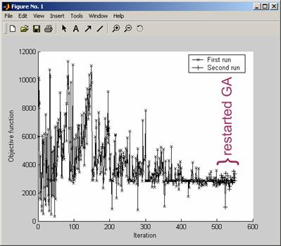
Figure 25 A Genetic Algorithm restarted following 500 iterations is already adapted to the objective function surface
5.16 What is the meaning of the optional control parameters?
Table 1 contains the meaning and default value of the optional control parameters. Since the meaning of the control parameters may differ depending upon the optimisation method in use the control parameters are organised with respect to the optimisation method.
|
Optimisation Method |
Control Parameter |
Meaning |
Default value |
|
Response Surface Modelling |
FUSION_TYP |
Flag to indicate RSM fusion type (differences=0, ratios=1) |
0 |
|
|
CST_BAD_PT |
The outer limit of acceptable constraint function values in RSMs |
None |
|
|
OBJ_BAD_PT |
The outer limit of acceptable objective function values in RSMs |
None |
|
|
RSM_EIF_W |
The weighting between exploitation and exploration used when applying expected improvement methods in RSM |
None |
|
|
RSM_NCSKIP |
Number of radial basis functions skipped for constraints |
0 |
|
|
RSM_NSKIP |
Number of radial basis functions skipped for objective function |
0 |
|
|
RSM_NULL_T |
Percentage worsening required in RBF regression to halt fitting |
10% |
|
1.1 OPTIVAR routine ADRANS |
OPT_TOL |
The accuracy with which solutions are found |
0 |
|
|
OPT_CTOL |
The accuracy with which constraints must be met to be considered satisfied |
0.001 |
|
|
OPT_STEP |
The step size used |
0.02 |
|
|
OVR_MAND |
Turns on mandatory design constraints |
0 (off) |
|
|
OVR_PENAL |
Selects the kind of penalty function used by a number of the OPTIVAR routines: 1 = one pass external 2 = Fiacco-McCormick 3 = Powell 4 = Schuldt |
1 |
|
|
OVR_SEED |
Sets the seed for random number sequences |
128 |
|
1.2 OPTIVAR routine DAVID |
OPT_TOL |
The accuracy with which solutions are found |
0 |
|
|
OPT_CTOL |
The accuracy with which constraints must be met to be considered satisfied |
0.001 |
|
|
OPT_STEP |
The step size used |
1.00E-06 |
|
|
OVR_MAND |
Turns on mandatory design constraints |
0 (off) |
|
|
OVR_PENAL |
Selects the kind of penalty function used by a number of the OPTIVAR routines: 1 = one pass external 2 = Fiacco-McCormick 3 = Powell 4 = Schuldt |
1 |
|
|
OVR_CONV |
Sets the convergence criterion |
1D-4/1D-5 |
|
1.3 OPTIVAR routine FLETCH |
OPT_TOL |
The accuracy with which solutions are found |
0 |
|
|
OPT_CTOL |
The accuracy with which constraints must be met to be considered satisfied |
0.001 |
|
|
OPT_STEP |
The step size used |
1.00E-06 |
|
|
OVR_MAND |
Turns on mandatory design constraints |
0 (off) |
|
|
OVR_PENAL |
Selects the kind of penalty function used by a number of the OPTIVAR routines: 1 = one pass external 2 = Fiacco-McCormick 3 = Powell 4 = Schuldt |
1 |
|
|
OVR_CONV |
Sets the convergence criterion |
1D-4/1D-5 |
|
1.4 OPTIVAR routine JO |
OPT_TOL |
The accuracy with which solutions are found |
0 |
|
|
OPT_CTOL |
The accuracy with which constraints must be met to be considered satisfied |
1.00E-03 |
|
|
OPT_STEP |
The step size used |
1.00E-06 |
|
|
OVR_MAND |
Turns on mandatory design constraints |
0 (off) |
|
|
OVR_PENAL |
Selects the kind of penalty function used by a number of the OPTIVAR routines: 1 = one pass external 2 = Fiacco-McCormick 3 = Powell 4 = Schuldt |
1 |
|
|
OVR_CONV |
Sets the convergence criterion |
1D-4/1D-5 |
|
1.5 OPTIVAR routine PDS |
OPT_TOL |
The accuracy with which solutions are found |
0 |
|
|
OPT_CTOL |
The accuracy with which constraints must be met to be considered satisfied |
1.00E-03 |
|
|
OPT_STEP |
The step size used |
0.1 |
|
|
OVR_MAND |
Turns on mandatory design constraints |
0 (off) |
|
|
OVR_PENAL |
Selects the kind of penalty function used by a number of the OPTIVAR routines: 1 = one pass external 2 = Fiacco-McCormick 3 = Powell 4 = Schuldt |
1 |
|
|
OVR_CONV |
Sets the convergence criterion |
1D-4/1D-5 |
|
1.6 OPTIVAR routine SEEK |
OPT_TOL |
The accuracy with which solutions are found |
0 |
|
|
OPT_CTOL |
The accuracy with which constraints must be met to be considered satisfied |
1.00E-03 |
|
|
OPT_STEP |
The step size used |
0.01 |
|
|
OVR_MAND |
Turns on mandatory design constraints |
0 (off) |
|
|
OVR_PENAL |
Selects the kind of penalty function used by a number of the OPTIVAR routines: 1 = one pass external 2 = Fiacco-McCormick 3 = Powell 4 = Schuldt |
1 |
|
|
OVR_STOP |
sets the minimum step length stopping criterion |
0.01 |
|
1.7 OPTIVAR routine SIMPLX |
OPT_TOL |
The accuracy with which solutions are found |
0 |
|
|
OPT_CTOL |
The accuracy with which constraints must be met to be considered satisfied |
1.00E-03 |
|
|
OPT_STEP |
The step size used |
0.1 |
|
|
OVR_MAND |
Turns on mandatory design constraints |
0 (off) |
|
|
OVR_PENAL |
Selects the kind of penalty function used by a number of the OPTIVAR routines: 1 = one pass external 2 = Fiacco-McCormick 3 = Powell 4 = Schuldt |
1 |
|
|
OVR_CONV |
Sets the convergence criterion |
1D-4/1D-5 |
|
1.8 OPTIVAR routine APPROX |
OPT_TOL |
The accuracy with which solutions are found |
0 |
|
|
OPT_CTOL |
The accuracy with which constraints must be met to be considered satisfied |
1.00E-03 |
|
|
OPT_STEP |
The step size used |
0.001 |
|
|
OVR_MAND |
Turns on mandatory design constraints |
0 (off) |
|
|
OVR_PENAL |
Selects the kind of penalty function used by a number of the OPTIVAR routines: 1 = one pass external 2 = Fiacco-McCormick 3 = Powell 4 = Schuldt |
1 |
|
|
OVR_STEP |
Sets the fraction of range limiting step lengths |
0.1 |
|
|
OVR_SIMP |
Sets the maximum number of simplex iterations |
46 |
|
1.9 OPTIVAR routine RANDOM |
OPT_TOL |
The accuracy with which solutions are found |
0 |
|
|
OPT_CTOL |
The accuracy with which constraints must be met to be considered satisfied |
1.00E-03 |
|
|
OPT_STEP |
The step size used |
0.02 |
|
|
OVR_MAND |
Turns on mandatory design constraints |
0 (off) |
|
|
OVR_PENAL |
Selects the kind of penalty function used by a number of the OPTIVAR routines: 1 = one pass external 2 = Fiacco-McCormick 3 = Powell 4 = Schuldt |
1 |
|
|
OVR_NPTS |
Sets the number of points retained per iteration |
5 |
|
|
OVR_SHRK |
Sets the shrinkage factor |
4 |
|
2.3 NAG routine E04UCF |
NAG_BIGBND |
Sets the size of non-existent upper bounds. |
1.00E+10 |
|
|
NAG_ETA |
Sets the accuracy of the linear minimizations |
0.5 |
|
|
NAG_RHO |
Used in the definition of the augmented Lagrangian function |
1 |
|
|
OPT_TOL |
The accuracy with which solutions are found |
0 |
|
|
OPT_CTOL |
The accuracy with which constraints must be met to be considered satisfied |
1.00E-03 |
|
|
OPT_STEP |
The step size used |
5.0N |
|
|
MC_MAND |
Turns on mandatory design constraints |
0 (off) |
|
2.4 bit climbing |
BC_NBIN |
The number of bits used per variable in binary discretisation |
12 |
|
|
BC_PENAL |
Set the penalty function control parameter, r, with values less than one invoking the modified Fiacco and McCormick function (OPTIM2) otherwise the one pass method is used (OPTIM1) |
1.00E+20 |
|
|
BC_NRANDM |
The number of random numbers drawn and discarded before starting the optimiser |
0 |
|
|
OPT_TOL |
The accuracy with which solutions are found |
0 |
|
|
OPT_CTOL |
The accuracy with which constraints must be met to be considered satisfied |
1.00E-03 |
|
|
OPT_STEP |
The step size used |
1.00E-05 |
|
|
MC_MAND |
Turns on mandatory design constraints |
0 (off) |
|
2.5 dynamic hill climbing |
DHC_INITSZ |
Sets the non-dimensional size of the initial steps in the hill climbing search |
0.5 |
|
|
DHC_THRESH |
The hill climbing searches proceed with reducing step sizes until they are less than the value set by this parameter |
0.01 |
|
|
DHC_PENAL |
Sets the penalty function control parameter, r, with values less than one invoking the modified Fiacco and McCormick function (OPTIM2) otherwise the one pass method is used (OPTIM1) |
1.00E+20 |
|
|
DHC_NRANDM |
The number of random numbers drawn and discarded before starting the optimiser |
0 |
|
|
OPT_TOL |
The accuracy with which solutions are found |
0 |
|
|
OPT_CTOL |
The accuracy with which constraints must be met to be considered satisfied |
1.00E-03 |
|
|
OPT_STEP |
The step size used |
1.00E-05 |
|
|
MC_MAND |
Turns on mandatory design constraints |
0 (off) |
|
2.6 population based incremental learning |
PL_NBIN |
The number of bits used per variable in binary discretisation |
12 |
|
|
PL_NPOP |
The number of random guesses |
100 |
|
|
PL_PENAL |
Sets the penalty function control parameter, r, with values less than one invoking the modified Fiacco and McCormick function (OPTIM2) otherwise the one pass method is used (OPTIM1) |
1.00E+20 |
|
|
PL_LRATE |
The learning rate controls how rapidly the probability vector changes towards the successful solutions at the end of each generation |
0.05 |
|
|
PL_PMUTNT |
mutation is applied to the probability vector randomly at the end of each generation with this probability per element |
0.02 |
|
|
PL_NRANDM |
The number of random numbers drawn and discarded before starting the optimiser |
0 |
|
|
OPT_TOL |
The accuracy with which solutions are found |
0 |
|
|
OPT_CTOL |
The accuracy with which constraints must be met to be considered satisfied |
1.00E-03 |
|
|
OPT_STEP |
The step size used |
1.00E-05 |
|
|
MC_MAND |
Turns on mandatory design constraints |
0 (off) |
|
2.7 numerical recipes routines |
OPT_TOL |
The accuracy with which solutions are found |
0 |
|
|
OPT_CTOL |
The accuracy with which constraints must be met to be considered satisfied |
1.00E-03 |
|
|
OPT_STEP |
The step size used |
1.00E-05 |
|
|
MC_MAND |
Turns on mandatory design constraints |
0 (off) |
|
|
MC_TYPE |
Selects the kind of optimizer used by the numerical recipes routines: 1 = Powell 2 = Polak-Ribiere 3 = Fletcher-Reeves 4 = Broyden-Fletcher |
1 |
|
|
MC_PENAL |
Selects the kind of penalty function used by the numerical recipes routines: 1 = one pass external 2 = Fiacco-McCormick |
1 |
|
2.8 design of experiment based routines |
DOE_NRANDM |
DoE sequence random number seed |
|
|
|
MC_TYPE |
DoE search methods: 1 = Random 2 = Lptau 3 = Central composite + Lptau 4 = Full factorial + Lptau 5 = Latin hypercubes 6 = Cell-based latin hypercubes 7 = User supplied candidate points |
1 |
|
|
MC_MAND |
Turns on mandatory design constraints |
0 (off) |
|
2.9 design of experiment based routines (without function calls) |
DOE_NRANDM |
Six Design of Experiment search methods |
0 |
|
|
MC_MAND |
Turns on mandatory design constraints |
0 (off) |
|
3.11 Schwefel library Fibonacci search |
OPT_TOL |
The accuracy with which solutions are found |
0 |
|
|
OPT_CTOL |
The accuracy with which constraints must be met to be considered satisfied |
1.00E-03 |
|
|
OPT_STEP |
The step size used |
1.00E-05 |
|
|
SC_PENAL |
Selects the kind of penalty function used by unconstrained search methods in the Schwefel library routines: 1 = one pass external 2 = Fiacco-McCormick |
1 |
|
3.12 Schwefel library Golden section search |
OPT_TOL |
The accuracy with which solutions are found |
0 |
|
|
OPT_CTOL |
The accuracy with which constraints must be met to be considered satisfied |
1.00E-03 |
|
|
OPT_STEP |
The step size used |
1.00E-05 |
|
|
SC_PENAL |
Selects the kind of penalty function used by unconstrained search methods in the Schwefel library routines: 1 = one pass external 2 = Fiacco-McCormick |
1 |
|
3.13 Schwefel library Lagrange interval search |
OPT_TOL |
The accuracy with which solutions are found |
0 |
|
|
OPT_CTOL |
The accuracy with which constraints must be met to be considered satisfied |
1.00E-03 |
|
|
OPT_STEP |
The step size used |
1.00E-05 |
|
|
SC_PENAL |
Selects the kind of penalty function used by unconstrained search methods in the Schwefel library routines: 1 = one pass external 2 = Fiacco-McCormick |
1 |
|
3.2 Schwefel library Hooke and Jeeves search |
OPT_TOL |
The accuracy with which solutions are found |
0 |
|
|
OPT_CTOL |
The accuracy with which constraints must be met to be considered satisfied |
1.00E-03 |
|
|
OPT_STEP |
The step size used |
1.00E-05 |
|
|
SC_PENAL |
Selects the kind of penalty function used by unconstrained search methods in the Schwefel library routines: 1 = one pass external 2 = Fiacco-McCormick |
1 |
|
3.3 Schwefel library Rosenbrock search |
OPT_TOL |
The accuracy with which solutions are found |
0 |
|
|
OPT_CTOL |
The accuracy with which constraints must be met to be considered satisfied |
1.00E-03 |
|
|
OPT_STEP |
The step size used |
1.00E-05 |
|
3.41 Schwefel library DSCG search |
OPT_TOL |
The accuracy with which solutions are found |
1.00E-03 |
|
|
OPT_CTOL |
The accuracy with which constraints must be met to be considered satisfied |
1.00E-03 |
|
|
OPT_STEP |
The step size used |
1.00E-05 |
|
|
SC_PENAL |
Selects the kind of penalty function used by unconstrained search methods in the Schwefel library routines: 1 = one pass external 2 = Fiacco-McCormick |
1 |
|
3.42 Schwefel library DSCP search |
OPT_TOL |
The accuracy with which solutions are found |
0 |
|
|
OPT_CTOL |
The accuracy with which constraints must be met to be considered satisfied |
1.00E-03 |
|
|
OPT_STEP |
The step size used |
1.00E-05 |
|
|
SC_PENAL |
Selects the kind of penalty function used by unconstrained search methods in the Schwefel library routines: 1 = one pass external 2 = Fiacco-McCormick |
1 |
|
3.5 Schwefel library Powell search |
OPT_TOL |
The accuracy with which solutions are found |
0 |
|
|
OPT_CTOL |
The accuracy with which constraints must be met to be considered satisfied |
1.00E-03 |
|
|
OPT_STEP |
The step size used |
1.00E-05 |
|
|
SC_PENAL |
selects the kind of penalty function used by unconstrained search methods in the Schwefel library routines : 1 = one pass external 2 = Fiacco-McCormick |
1 |
|
|
SC_TYPE |
Selects the default convergence criterion or an alternate criterion: 1 = default convergence 2 = alternate convergence |
1 |
|
3.6 Schwefel library DFPS search |
OPT_TOL |
The accuracy with which solutions are found |
0 |
|
|
OPT_CTOL |
The accuracy with which constraints must be met to be considered satisfied |
1.00E-03 |
|
|
OPT_STEP |
The step size used |
1.00E-05 |
|
|
SC_PENAL |
Selects the kind of penalty function used by unconstrained search methods in the Schwefel library routines: 1 = one pass external 2 = Fiacco-McCormick |
1 |
|
|
SC_CONV |
Defines the expected solution value of the objective function at the optimum, default zero (50% improvement) |
0 |
|
3.7 Schwefel library Simplex search |
OPT_TOL |
The accuracy with which solutions are found |
1.00E-03 |
|
|
OPT_CTOL |
The accuracy with which constraints must be met to be considered satisfied |
1.00E-03 |
|
|
OPT_STEP |
The step size used |
1.00E-05 |
|
|
SC_PENAL |
Selects the kind of penalty function used by unconstrained search methods in the Schwefel library routines: 1 = one pass external 2 = Fiacco-McCormick |
1 |
|
|
SC_NITERS |
The number of iterations before convergence testing is applied, default zero (the total number of function calls to be used divided by 25 times the number of design variables) |
0 |
|
3.8 Schwefel library Complex search |
OPT_TOL |
The accuracy with which solutions are found |
0 |
|
|
OPT_CTOL |
The accuracy with which constraints must be met to be considered satisfied |
1.00E-03 |
|
|
OPT_STEP |
The step size used |
1.00E-05 |
|
|
SC_PENAL |
Selects the kind of penalty function used by unconstrained search methods in the Schwefel library routines: 1 = one pass external 2 = Fiacco-McCormick |
1 |
|
3.91 Schwefel library two-membered evolution strategy (EVOL) |
SC_LS |
How severe convergence testing is, with bigger values requiring the objective function to remain essentially stationary for longer before convergence is considered complete |
2 |
|
|
SC_NRANDM |
The number of random numbers drawn and discarded before starting the optimiser |
0 |
|
|
OPT_TOL |
The accuracy with which solutions are found |
1.00E-03 |
|
|
OPT_CTOL |
The accuracy with which constraints must be met to be considered satisfied |
1.00E-03 |
|
|
OPT_STEP |
The step size used |
1.00E-05 |
|
|
SC_LR |
Controls step size management, with bigger values giving a slower but more accurate search |
1 |
|
|
SC_SN |
Controls step size adjustment, which can be kept constant using a value of unity |
0.85 |
|
3.92 Schwefel library multi-membered evolution strategy (KORR) |
SC_IELTER |
The number of parents in a generation |
10 |
|
|
SC_NACHKO |
The number of descendants of a generation |
100 |
|
|
SC_NS |
The number of different step size parameters |
N |
|
|
SC_DELS |
The global random step sizes |
1/sqtr(2N) |
|
|
SC_DELI |
The local random step sizes |
1/sqtr(2N)/sqtr(NS) |
|
|
SC_DELP |
The correlation ellipsoid angles |
5 × 0. 01745 = 5° |
|
|
SC_BKORRL |
Switches on the rotation of the correlation ellipsoid if non-zero |
1 |
|
|
SC_KONVKR |
Number of generations used when applying convergence tests |
1 |
|
|
SC_NRANDM |
The number of random numbers drawn and discarded before starting the optimiser |
0 |
|
|
OPT_TOL |
The accuracy with which solutions are found |
0 |
|
|
OPT_CTOL |
The accuracy with which constraints must be met to be considered satisfied |
1.00E-03 |
|
|
OPT_STEP |
The step size used |
1.00E-05 |
|
|
SC_TYPE |
Controls whether the "comma" or "plus" version of the code is used: 1 = comma 2 = plus |
1 |
|
|
SC_IREKOM |
Controls the recombination type (n.b., each digit in this variable must lie between 1 and 5) |
333 |
|
4 genetic algorithm search |
GA_NBIN |
The number of bits used per variable in binary discretisation |
12 |
|
|
GA_NPOP |
Population size each generation |
50 |
|
|
GA_PENAL |
Set the penalty function control parameter, r, with values less than one invoking the modified Fiacco and McCormick function (OPTIM2) otherwise the one pass method is used (OPTIM1) |
1.00E+20 |
|
|
GA_PBEST |
The proportion of the solutions that are used to form the parents of the next generation |
0.8 |
|
|
GA_PCROSS |
The proportion of the solutions in the population that are crossed to form new solutions |
0.8 |
|
|
GA_PINVRT |
The proportion of the solutions in the population that have their ordering codes inverted to form new solutions |
0.2 |
|
|
GA_PMUTNT |
Mutation is allowed at a level set by this parameter, i.e., this fraction of the total number of binary digits are reversed at each pass (n.b. greater than 0.5 results in randomisation) |
0.005 |
|
|
GA_PRPTNL |
If .TRUE. the make-up of the following generation is then biased in favour of the most successful according to their objective function values, otherwise survival is proportional to ranking but scaled to prevent dominance and stagnation |
1 (.TRUE.) |
|
|
GA_ALPHA |
The cluster penalising function. Small values giving less severe penalties than those nearer one, and a value less than zero turning the mechanism off |
0.2 |
|
|
GA_DMIN |
The minimum distance between cluster centroids |
0.05 |
|
|
GA_DMAX |
The furthest distance a new solution can be from an existing cluster centroid without a new cluster being formed |
0.2 |
|
|
GA_NCLUST |
The initial number of clusters, either in absolute terms or, if it is < 1. 0, as a fraction of the population size |
0.1 |
|
|
GA_NBREED |
Breeding is restricted to be between members of the same cluster if there are at least this many members in the cluster |
0.1 |
|
|
GA_PSEED |
Seeding of the initial, randomly generated members of the population is allowed at a level set by this parameter (0 = random, 1.0 clones of initial point) |
0 |
|
|
GA_NRANDM |
The number of random numbers drawn and discarded before starting the optimiser |
0 |
|
5 simulated annealing |
SA_NBIN |
The number of bits used per variable in binary discretisation |
12 |
|
|
SA_PTEMP |
The power to which the number of iterations must be raised to calculate the number of annealing temperatures |
1/3 |
|
|
SA_PWIDTH |
The range of temperatures in the annealing schedule, with large values giving a wide range of temperatures, which carries the risk of rapid freezing but gives a wider ranging search |
5 |
|
|
SA_PCOLD |
The bottom temperature in the annealing schedule, with values over two giving lower temperatures and thus more accurate results at the expense of perhaps missing the global optimum |
2 |
|
|
SA_SCHED |
If this parameter exists and contains an array of variables it is taken to be a cooling schedule which is to be used in place of the preceding three parameters |
|
|
|
SA_PENAL |
Sets the penalty function control parameter, r, with values less than one invoking the modified Fiacco and McCormick function (OPTIM2) otherwise the one pass method is used (OPTIM1) |
1.00E+20 |
|
|
SA_PMUTNT |
Mutation is allowed at a level set by this parameter, i.e., this fraction of the total number of binary digits are reversed at each evaluation (setting SA_PMUTNT negative causes the mutations to be made to the actual variables rather than the binary digits) |
0.1 |
|
|
SA_NRANDM |
The number of random numbers drawn and discarded before starting the optimiser |
0 |
|
6 evolutionary programming |
EP_NBIN |
The number of bits used per variable in binary discretisation |
12 |
|
|
EP_NPOP |
Population size each generation |
50 |
|
|
EP_PENAL |
Set the penalty function control parameter, r, with values less than one invoking the modified Fiacco and McCormick function (OPTIM2) otherwise the one pass method is used (OPTIM1) |
1.00E+20 |
|
|
EP_IMUTNT |
Mutation is controlled so that the best members are mutated least and the worst, most, this parameter governs the order of the mutation with ranking, a value of one thus gives a linear change, two a quadratic one and so on (only positive values being allowed), default two; |
2 |
|
|
EP_TOURN |
The number of members in the ranking tournament, either in absolute terms or, if it is < 1. 0, as a fraction of the population size |
0.5 |
|
|
EP_NRANDM |
The number of random numbers drawn and discarded before starting the optimiser |
0 |
|
7 evolution strategy |
ES_NPPOP |
The population size |
100 |
|
|
ES_NCPOP |
The parent populations size, a fraction of the total population size |
1 |
|
|
ES_PENAL |
Sets the penalty function control parameter, r, with values less than one invoking the modified Fiacco and McCormick function (OPTIM2) otherwise the one pass method is used (OPTIM1) |
1.00E+20 |
|
|
ES_DELSIG |
Used to set the standard deviation of a random number whose exponential is then used to scale the previous mutation control parameter. |
0.1 |
|
|
ES_UCHILD |
When selecting the next generation all the children may be used or a mixture of the best children and parents used; if this parameter is non-zero it is taken to be .TRUE. and the children are used in preference to parents. |
0 (false) |
|
|
ES_VDSCRT |
Controls the crossover type between parents for design variables. Either discrete crossover (.TRUE.) or intermediate crossover (.FALSE.). |
1 (true) |
|
|
ES_MDSCRT |
Controls the crossover type between parents for mutation control parameters. Either discrete crossover (.TRUE.) or intermediate crossover (.FALSE.). |
0 (false) |
|
|
ES_NRANDM |
The number of random numbers drawn and discarded before starting the optimiser |
0 |
Table 1 OptionsMatlab optional control parameters
5.17 How do I deal with failed calculations when constructing a response surface model?
Failures may occur when calculating the value of an objective function during a direct search. These failures may be stochastic (perhaps due to the unexpected failure of a Grid resource), or they may be indicative of a problematic area of the parameter space (perhaps representing an unfeasible geometry). There are a couple of possible strategies to ensure that failed calculations are correctly handled by OptionsMatlab when constructing and searching a Response Surface Model.
The optional control parameter OBJ_BAD_PT may be used to define an outer bound for acceptable values of an objective function. When OptionsMatlab encounters objective function values exceeding OBJ_BAD_PT during the construction of a Response Surface Model these values will be ignored. During minimisation OptionsMatlab will ignore any objective function values greater than OBJ_BAD_PT, whereas during maximisation values less than OBJ_BAD_PT will be ignored.
It is possible to use OBJ_BAD_PT to filter stochastic failures that occur during the evaluation of the objective function. For a minimisation problem the Matlab function defining the user's objective function should return a very large value for the objective function (which exceeds expected values) upon failure. When building and searching a Response Surface Model of the objective function the OptionsMatlab input structure should contain the field OBJ_BAD_PT with a value less than that of the failed calculations. The bad points will therefore not influence the Response Surface Model of the objective function.
When a failed calculation represents a problematic area of the parameter space it is sometimes desirable to steer a design search away from these areas. To do this it is possible to define an extra constraint to indicate bad points. In this case when a calculation fails this constraint should be set to indicate an invalid point. As the design search proceeds the constraint may steer the optimiser away from these problematic areas. When searching over a Response Surface Model this strategy may be used in conjunction with OBJ_BAD_PT.
5.18 How do I build and evaluate a RSM faster?
There are a number of ways to make OptionsMatlab run faster when building and evaluating a Response Surface Model.
If additional output information is requested from OptionsMatlab (OLEVEL>0) further calculations may be performed. This may significantly increase the time taken to build and evaluate a RSM, in particular for large datasets. Therefore to perform faster searches of a RSM it may be advantageous to set OLEVEL=0 in the OptionsMatlab input structure.
When performing multiple searches of a Stochastic Process Model (SPM), i.e. when OBJMOD or CONMOD equal to 4.1, 4.2 or 4.3, it is possible to avoid rebuilding the SPM by passing the hyper-parameters for the model in the input structure. When a SPM is first built and searched (or when the hyper-parameters are explicitly tuned, see section 5.11) the hyper-parameters are returned in the output structure fields OBJHYPER (and/or CONHYPER). By adding these fields to the OptionsMatlab input structure when subsequently searching the SPM the hyper-parameters will not be rebuilt. However, please note that it is important to rebuild the hyper-parameters following changes to dataset otherwise they may become ill-defined for your dataset.
Copyright © 2007, The Geodise Project, University of Southampton