[Advanced] Geophysical processing and interpretation exercises
I thought it might be nice to provide an [Advanced] supplementary exercise for learners on the Archaeology of Portus course. Please be aware that this is additional content and so doesn’t form any part of the official course. We might work it in in the future but for now it is hopefully a fun way to take your studies further. You are very welcome to do this exercise whether you are enrolled or not (and you can still register on the course for free), but you will find relevant information to support this exercise in the following sections of the FutureLearn course:
- Introducing landscape approaches to the port
- [Advanced] Studying the hinterland of Portus
- Geophysical prospection
- Combining different methods
If you are registered on the course then please post comments and queries there on the Geophysical prospection step rather than on this blog post, so that other learners will see them. Best wishes, Kristian Strutt
Part One: Geophysical Data Processing
As part of the daily work of surveying an archaeological site using geophysical techniques, the surveyors need to download the data at the end of the day, to check that there are no issues with it and to begin processing the data to remove any variations or anomalies caused by operator error or external effects that are not due to archaeological remains. With magnetometry the main types or interference that may occur are usually down to the presence of iron (ferrous) material. This could be due to the operator of the survey instrument carrying something metallic on their person, or iron objects in the plough-soil of the area being surveyed. In addition to variations in the earth’s magnetic field can cause the instrument to ‘drift’ creating an effect on the data.
Some of these issues cannot be processed out, and survey grids may need to be resurveyed if the effect is extreme. Some problematic variations in the data can, however, be processed out, providing a clearer representation of potential archaeological features. To see how geophysical survey data is organised, and to see the types of process that are used on data, some grids of magnetometer data have been uploaded onto this website. We use professional software to process survey data, which can require expensive licences. There is, however, a freeware version of geophysical software called ‘Snuffler’ which will allow anyone to process survey data. To have a go at data processing simply download the survey grids from the website, then go to http://www.sussexarch.org.uk/geophys/snuffler.html and download and install Snuffler. There are help sections on the Snuffler website to help you do this.
Processing the magnetometry data using “snuffler”
- Download the sample dataset. You can download the XYZ data file via this link. When you have downloaded the file to your computer you need to rename the file AREA21D_sn.xyz
- To process the sample dataset you need to open Snuffler, having installed it on your computer. The link to downloading the software is in the previous section.
- You then need to create a new project under the file menu. Once created you open the project.
- Once open you need to import the xyz dataset that you downloaded and renamed above. It must be renamed AREA21D_sn.xyz. To import the data go to the file menu option and select import, then easy xyz import into new file then locate and find your AREA21D_sn.xyz file. Note, you will need to change the file type to be all files to view the xyz file.
- This opens the easy import box. The file name will be given at the top. Please select the dummy reading value to be 2047.5 (Geoplot). The dummy value in a dataset shows where no measurement was taken in the field. You cannot use zero, as with magnetometer data the values range between positive and negative, so zero is an actual value that may occur in a dataset. Therefore a spurious high value is used to represent dummy data, in this case 2047.5.
- Once you have done this then click okay and the data will be imported.
- To locate the data look at the side menu, and click on the project and double click on the data to open the file. This will appear as a series of numbers showing the location of individual values in the data.
- To continue using Snuffler to process the data please follow the Snuffler help section located under Help on the menu bar. I will mention a couple of other things here but the help section will be most useful.
- To view the data as a greyscale image rather then numbers, right click on the file in the lefthand menu window and select preview window. This will create a window allowing you to preview the magnetometer data as a greyscale. You should see a window with a greyscale image of two fields of data. Use the zoom in and zoom out icons on the toolbar to zoom in and out of the image.
- To process your data you need to create a view file. To do this right click on the data as you did to view the preview, then select spawn main view and save it with a name. This will create a new view, and a Filter menu will appear on the menu bar at the top.
Try some of the filter options. The most crucial would be to despike and destagger the data, perhaps to remove geology and then to interpolate:
- Despike – removes any extreme small scale readings in the data, the kind of thing caused by ferrous material in the ploughsoil.
- Destagger – removes any staggering in the data caused by walking the field collecting data in zigzag fashion, especially when dealing with difficult terrain.
- Remove Geology – will remove low frequency broad features. More applicable to res data as fluxgate gradiometers apply a filter function in the field.
- Interpolate – allows you to interpolate the data doubling the number of pixels in a particular direction. For instance with this data the pixels horizontally are 0.25m each, vertically they are 0.5m each, so you may want to interpolate vertically.
The best way to learn about these processes is to use the Snuffler Help section and try out different filters to attampt to get a clean and crisp image. This is the aim of the surveyor in conducting the fieldwork and processing the data.
Sharing your results
Try it out and please post your work onto the Portus Flickr group so that we can all have a look at your interpretations. If you are registered on the course then please post comments and queries there on the Geophysical prospection step rather than on this blog post, so that other learners will see them. Include a link to your Flickr images so we and other learners can provide feedback.
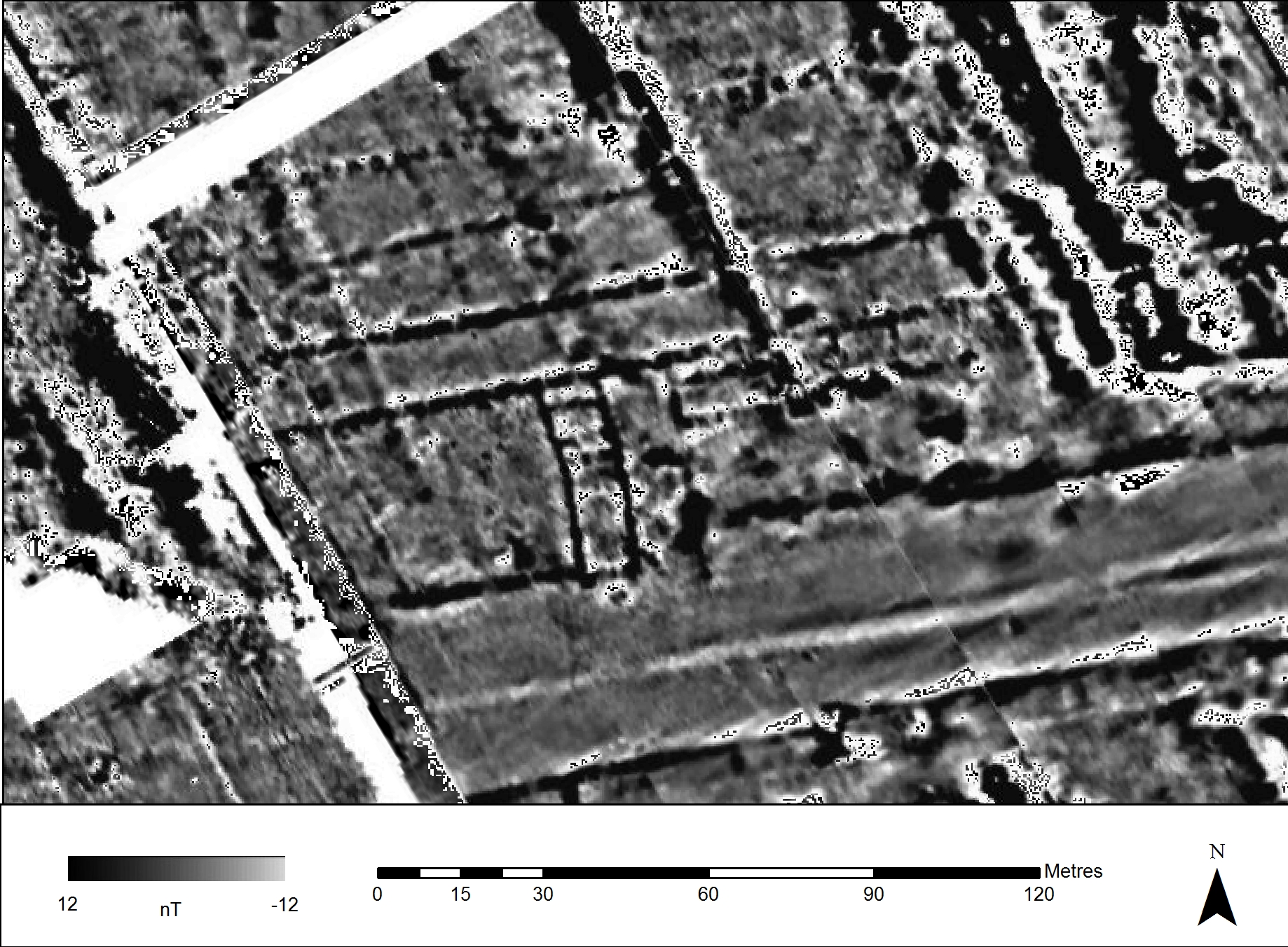
Part Two – Interpreting Magnetometer Data
Once the survey data has been processed, the surveyor must then produce a high resolution image of the data, and georeference the image with a map of the modern topography, ready to start the process of interpreting the data. The range of values in magnetometry span negative and positive values, for instance running from -12 to 12 nanotesla (nT). This range of values can be represented as a greyscale or colourscale, but are usually shown as the former, with shades from black (positive) to white (negative) being used. The archaeologist needs to scrutinise the image and produce an interpretation plan, showing his or her interpretation of what the different anomalies represent. In the past much of this was done using permatrace and a pen or pencil, drawing an interpretation over the printed survey image. Nowadays most archaeologists use computer software including GIS and drawing packages to do the work: digitising anomalies, setting parameters for each digitised line or polygon, and then changing the parameters of the symbols to create a shaded and coloured interpretation image. Some geophysicists still use the old fashioned methods, however, producing very accurate and detailed interpretations. For this second part of the exercise you should Download an image of an area of geophysics collected at Portus with a number of features running across it. The objective is for you to produce an interpretation of the results, either by printing our the image and tracing over it, or by using Paint or another type of software to digitise an interpretation. There are lots of free and low-priced drawing and painting tools online, including ones that allow you to load an image and trace over it. These exist for tablets as well as desktops and laptops.
Suggested activities
- Trace individual features that you think are significant.
- Label these with numbers or letters, and write a short interpretation of what you think they might be, using your labels to cross reference your text with your images. (You can include this in the image description if you upload your interpretation plans to Flickr).
- Discuss the range of data present in the image, and perhaps any problems visible.
Sharing your results
Please post your work onto the Portus Flickr group so that we can all have a look at your interpretations. If you are registered on the course then please post comments and queries there on the Geophysical prospection step rather than on this blog post, so that other learners will see them. Include a link to your Flickr images so we and other learners can provide feedback.
Examples of interpretations of different kinds of data
The following images produced by members of the Portus Project provide you with examples of interpreting geophysical data. Clicking on the image switches from the data to the interpretation, and vice versa.
Magnetometry
Click the map to toggle between the results and the interpretation
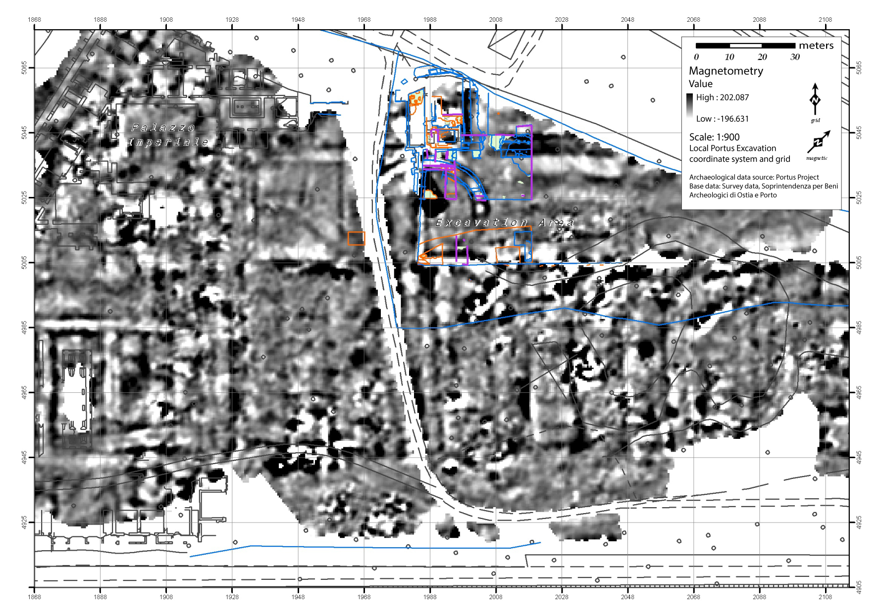
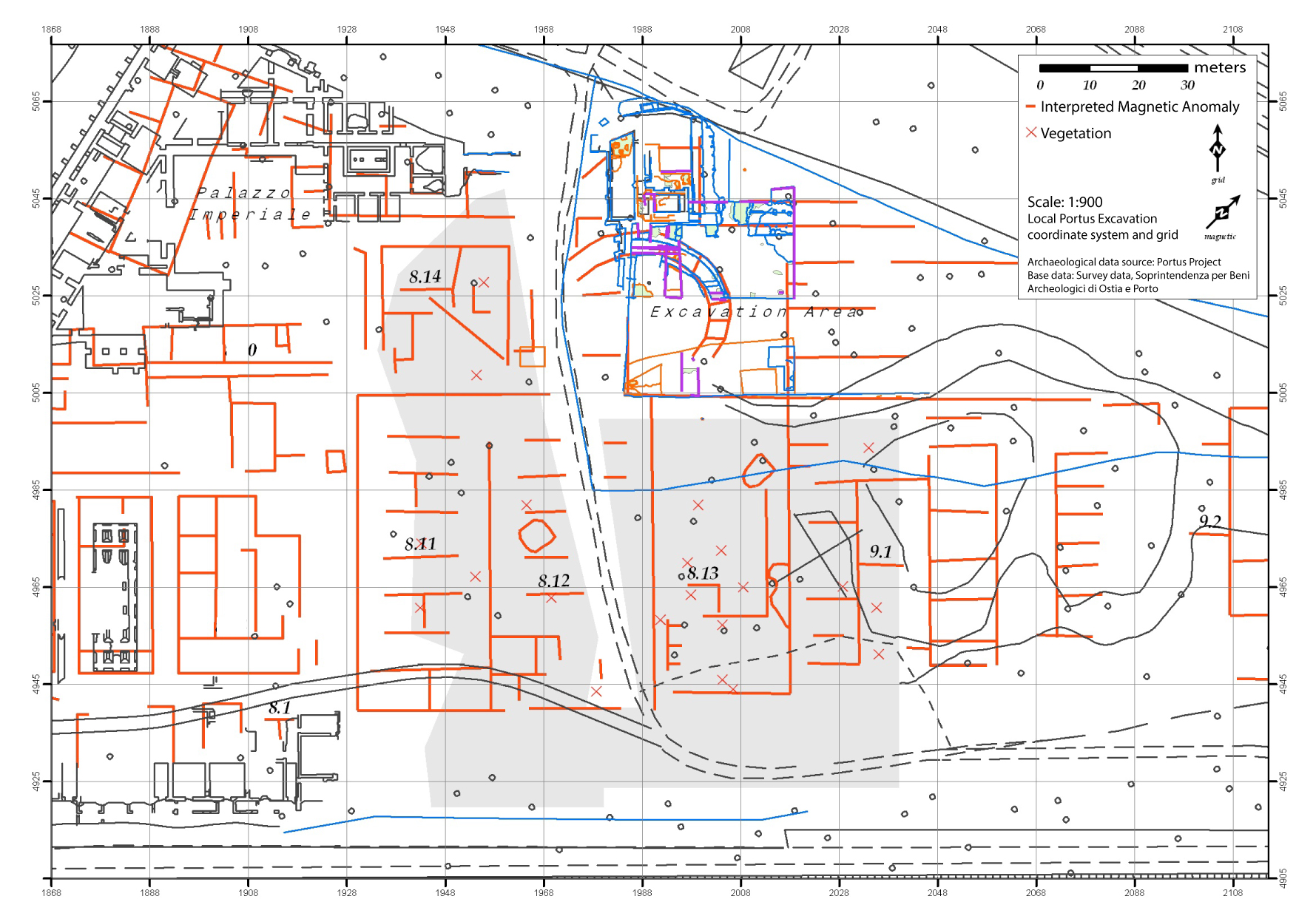
© Jessica Ogden, University of Southampton
Resistivity
Click the map to toggle between the results and the interpretation
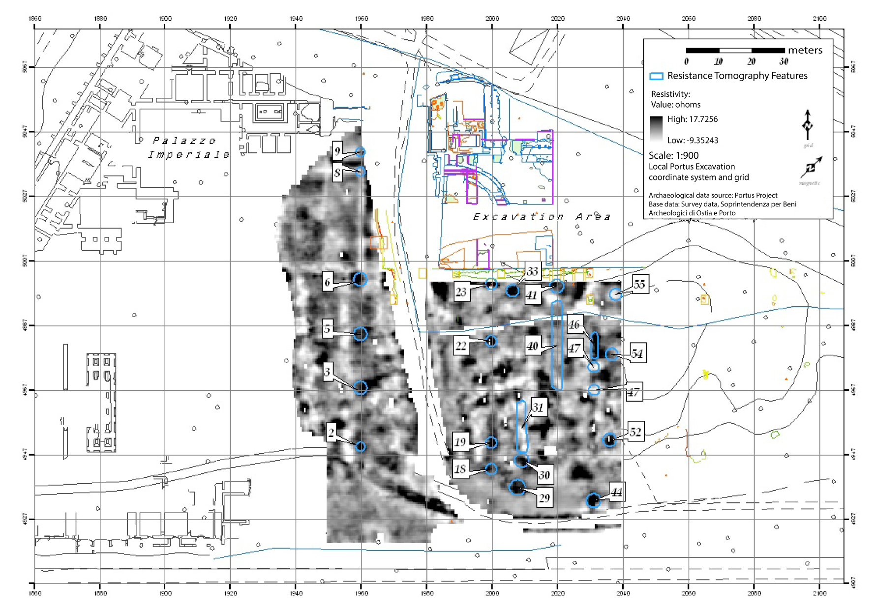
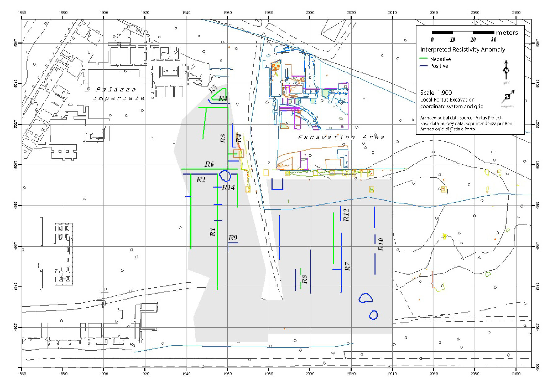
© Jessica Ogden, University of Southampton
Ground Penetrating Radar
Click the map to toggle between the results and the interpretation
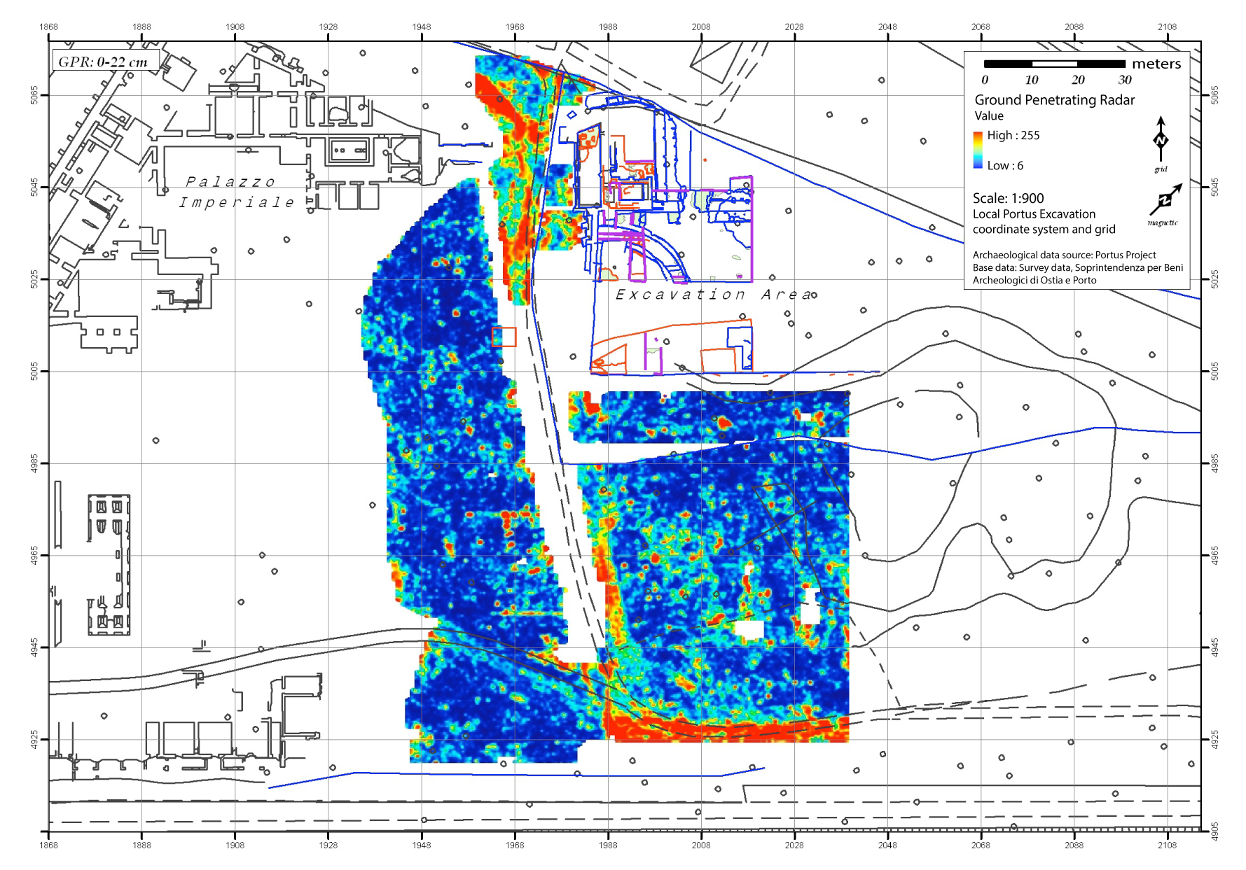
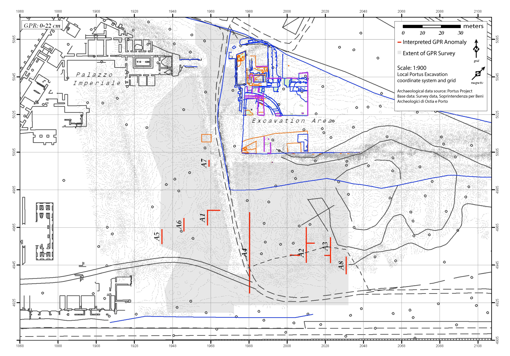
© Jessica Ogden, University of Southampton
Files to download
- XYZ data file (remember to rename AREA21D_sn.XYZ)
- Magnetometry sample grid file


